Train CNN

Train a Convolutional Neural Network

Introduction

We are now ready to bring the components we have been discussing together to train a convolutional neural network (CNN) to differentiate land cover types using the EuroSatAllBands dataset. In contrast to the fully connected example, we will now train the model using the images as opposed to the band means. Let’s jump into the workflow.

Preparation

First, I import the required packages as normal including numpy, pandas, matplotlib, os, and scikit-learn. From torch.utils.data, I import the DataSet and DataLoader classes. To load in multiband geospatial raster data, I will use rasterio. Assessment metrics will be implemented using torchmetrics. Lastly, I will apply data augmentations using torchvision.

I also set the device to the GPU. For training CNNs, it is generally best to use a GPU. Training on a CPU, especially when using a large dataset and/or a complex architecture, can be extremely slow or even untenable. For the remainder of this class, you will need access to a GPU in order to train models. As mentioned in prior modules, you can access GPUs using Google Colab, but there are some use limitations.

import numpy as np
import pandas as pd
import matplotlib
from matplotlib import pyplot as plt 

import os
from sklearn import preprocessing
from sklearn.metrics import confusion_matrix
from sklearn.metrics import classification_report


import torch
import torch.nn as nn
from torch.utils.data.dataset import Dataset
from torch.utils.data import DataLoader

import rasterio as rio

import torchmetrics as tm

import torchvision.transforms as transforms

device = torch.device("cuda:0" if torch.cuda.is_available() else "cpu")
print(device)

cuda:0

I next set the folder path to the EuroSatAllBands data on my local machine to a variable. You will need to change this directory to the appropriate path on your own machine. I then read in the data tables that were created in the DataSets and DataLoaders module as pandas DataFrames. There are separate tables for the training, validation, and testing data. Columns in the table provide the image name, path to each image, class name, and class numeric code. I am not recreating these tables here since they were already generated in a prior module. You may want to go back and review the DataSets and DataLoaders module for a refresher if you are struggling with these concepts.

folder = "C:/myFiles/work/dl/eurosat/EuroSATallBands/"

train = pd.read_csv(folder+"mytrain.csv")
test = pd.read_csv(folder+"mytest.csv")
val = pd.read_csv(folder+"myval.csv")

In order to normalize the data, I need to calculate the band means and standard deviations for the training samples. All of this code has already been explained in the DataSets and DataLoaders module, so I will not describe it in detail again here. Remember that it is generally best to normalize data using consistent means and standard deviations. Also, it is generally best to use only the training data to make these calculations to avoid a data leak. So, I will calculate the means and standard deviations from the training data, then use these values to normalize all three datasets. Here is a quick review of this process.

I define a DataSet subclass that allows me to read the data in batches. This is so that I can make use of PyTorch to obtain the statistics and so that I can work with these data in batches since the entire set is too large to process at once.
I then instantiate an instance of the DataSet subclass with the training samples as input.
I create a DataLoader to load the batches. Note that the batch size is set to 32 here. When reading entire images as opposed to band means, as I did for the fully connected neural network example, it is not possible to load a large set of images at once unless you are using multiple GPUs and/or have a lot of VRAM available. You may need to experiment with an appropriate batch size depending on your GPU hardware and available memory.
I define a function to calculate the means and standard deviations across batches and aggregate the results. This function was adapted from code provided at the link that is commented out.
I then run the function on the training DataLoader. Note that this may take several minutes to execute.

class EuroSat(Dataset):
    
    def __init__(self, df):
        super().__init__
        self.df = df
    
    def __getitem__(self, idx):
        image_name = self.df.iloc[idx, 1]
        label = self.df.iloc[idx, 3]
        label = np.array(label)
        source = rio.open(image_name)
        image = source.read()
        source.close()
        image = image.astype('float32')
        image = image[[1,2,3,4,5,6,7,8,11,12], :, :]
        image = torch.from_numpy(image)
        label = torch.from_numpy(label)
        label = label.long()
        return image, label 
        
    def __len__(self):
        return len(self.df)

trainDS = EuroSat(train)
print(len(trainDS))

trainDL = torch.utils.data.DataLoader(trainDS, batch_size=32, shuffle=True, sampler=None,
num_workers=0, pin_memory=False, drop_last=False)

#https://www.binarystudy.com/2021/04/how-to-calculate-mean-standard-deviation-images-pytorch.html
def batch_mean_and_sd(loader, inChn):
    
    cnt = 0
    fst_moment = torch.empty(inChn)
    snd_moment = torch.empty(inChn)

    for images, _ in loader:
        b, c, h, w = images.shape
        nb_pixels = b * h * w
        sum_ = torch.sum(images, dim=[0, 2, 3])
        sum_of_square = torch.sum(images ** 2,
                                  dim=[0, 2, 3])
        fst_moment = (cnt * fst_moment + sum_) / (cnt + nb_pixels)
        snd_moment = (cnt * snd_moment + sum_of_square) / (cnt + nb_pixels)
        cnt += nb_pixels

    mean, std = fst_moment, torch.sqrt(snd_moment - fst_moment ** 2)        
    return mean,std

band_stats = batch_mean_and_sd(trainDL, 10)

I am now ready to define the data pipeline to read the image chips and associated labels in batches and train the CNN. I begin by defining the DataSet subclass. This is the same DataSet subclass definition that was used in the DataSets and DataLoaders module. However, I have added some transforms, which we will discuss shortly. This requires adding another input parameter (transform). If the argument associated with this parameter is not None, then transforms will be applied. Using random data augmentations is one means to potentially combat overfitting. This is commonly employed when training CNNs. Let’s review the key components in this DataSet subclass.

The __init__() constructor method defines the input parameters. In this case, the user will be expected to input a DataFrame, band means, band standard deviations, and a data transforms object.
The __getitem__() method defines how each individual sample is loaded. This includes (1) reading the path to the image from the appropriate DataFrame column, (2) reading the numeric code from the appropriate DataFrame column and converting it to a numpy array, (3) reading the image using rasterio and the image name and path obtained from the DataFrame, (4) extracting out only the bands that I want to include as predictor variables, (5) normalizing the data by subtracting the band means then dividing by the band standard deviations, (6) converting the data to the 32-bit float type, (7) converting the numpy arrays representing the image and labels to torch tensors, (8) converting the numeric label tensor to a long integer data type, (9) applying transforms if they are provided, and (10) returning the image and numeric label as torch tensors with the expected data types and shapes.
The __len__() method returns the number of available samples.

class EuroSat(Dataset):
    
    def __init__(self, df, mnImg, sdImg, transform):
        self.df = df
        self.mnImg = mnImg
        self.sdImg = sdImg
        self.transform = transform
    
    def __getitem__(self, idx):
        image_name = self.df.iloc[idx, 1]
        label = self.df.iloc[idx, 3]
        label = np.array(label)
        source = rio.open(image_name)
        image = source.read()
        source.close()
        image = image[[1,2,3,4,5,6,7,8,11,12], :, :]
        image = np.subtract(image, self.mnImg)
        image = np.divide(image, self.sdImg)
        image = image.astype('float32')
        image = torch.from_numpy(image)
        label = torch.from_numpy(label)
        label = label.long()
        if self.transform is not None:
            image = self.transform(image)
        return image, label
        
    def __len__(self):
        return len(self.df)

The band means and standard deviations are converted to numpy arrays. I then convert these data to the correct shape for use in the processing pipeline. Specifically, the band means and standard deviations arrays are converted to a shape of (10, 64, 64). This correlates to the number of channels and the length of the spatial dimensions.

bndMns = np.array(band_stats[0].tolist())
bndSDs = np.array(band_stats[1].tolist())

mnImg = np.repeat(bndMns[0], 64*64).reshape((64,64,1))
for b in range(1,len(bndMns)):
    mnImg2 = np.repeat(bndMns[b], 64*64).reshape((64,64,1))
    mnImg = np.dstack([mnImg, mnImg2])
mnImg = np.transpose(mnImg, (2,0,1))

sdImg = np.repeat(bndSDs[0], 64*64).reshape((64,64,1))
for b in range(1,len(bndSDs)):
    sdImg2 = np.repeat(bndSDs[b], 64*64).reshape((64,64,1))
    sdImg = np.dstack([sdImg, sdImg2])
sdImg = np.transpose(sdImg, (2,0,1))

print(mnImg.shape)

(10, 64, 64)

print(sdImg.shape)

(10, 64, 64)

I now define some transforms that will be used to apply random data augmentations as a means to potentially combat overfitting. The Compose() function from torchvision allows you to define a series of transforms as a single object. The series of transforms must be provided as a list. Here, I am applying random horizontal and vertical flips of the images. The p parameter relates to the likelihood of the random alteration being applied; with this set to 0.3, there is a 30% chance of each transformation being applied.

There are many possible transformations. I recommend taking a look at the torchvision documentation: https://pytorch.org/vision/stable/transforms.html. It is not always clear what transformations should be applied, how often they should be applied, and the level of augmentation. For example, it is possible to apply sharpening, blurring, contrast enhancement, and desaturation. How much the image and associated DN values are augmented will depend on the provided settings. I generally try not to use extreme alterations. It generally takes some experimentation to determine what settings are adequate for a specific task and/or dataset. Again, the goal here is to potentially reduce overfitting and improve generalization of the resulting model by adding more variability to the training set. This makes it harder for the network to memorize the training data.

myTransforms = transforms.Compose(
    [transforms.RandomHorizontalFlip(p=0.3), 
    transforms.RandomVerticalFlip(p=0.3),]
    )

I now instantiate the DataSets and define the DataLoaders for the training and validation samples. In the training loop, the training samples will be used to train the model while the validation samples will be used to assess the model at the end of each training epoch. The testing samples will be used to assess the final model later in the module. They are not used within the training loop.

Both the training and validation datasets are being normalized using the statistics from the training data only in order to avoid a data leak. I am applying data augmentation transforms to the training data but not to the validation data since they will not be used to train the model or update the model parameters. It is not generally necessary or appropriate to apply data augmentations to the validation and testing data.

In the DataLoader, I set the batch size to 32, which worked well on my system. However, you may need to experiment with this to determine a batch size appropriate for your device. Remember that you can use multiple GPUs, if multiple GPUs are available. This was discussed in a prior module. In such cases, you can generally use a larger batch size. For the training data, I randomly shuffle the samples; however, this is not necessary for the validation data. I also drop the last batch for each set since a change in the batch size can be an issue.

trainDS = EuroSat(train, mnImg, sdImg, transform=myTransforms)
valDS = EuroSat(val, mnImg, sdImg, transform=None)

trainDL = torch.utils.data.DataLoader(trainDS, batch_size=32, shuffle=True, sampler=None,
num_workers=0, pin_memory=False, drop_last=True)

valDL = torch.utils.data.DataLoader(valDS, batch_size=32, shuffle=False, sampler=None,
num_workers=0, pin_memory=False, drop_last=True)

Check Batches and Data

It is generally recommended to check the data before using it to train or validate a model. I have printed some summary metrics for a batch of the training data and a single image from this batch. You can see that the shape of an image batch is (32, 10, 64, 64). The dimension order is batch, bands, height, and width. The shape of the labels is (32). This is a 1D tensor of 32 numeric codes, or one label for each image in the batch. The data type of the DN values in the image bands is 32-bit float. For the individual image, the band means make sense since the data have been normalized to z-scores. Lastly, the range of class numeric codes, 0 to 9, makes sense; this is because there are 10 classes. The data type of the class codes is long integer. In short, all of this looks good.

batch = next(iter(trainDL))
images, labels = batch
print(f'Batch Image Shape: {images.shape}, Batch Label Shape: {labels.shape}')

Batch Image Shape: torch.Size([32, 10, 64, 64]), Batch Label Shape: torch.Size([32])

print(f'Batch Image Data Type: {images.dtype}, Batch Label Data Type: {labels.dtype}')

Batch Image Data Type: torch.float32, Batch Label Data Type: torch.int64

print(f'Batch Image Band Means: {torch.mean(images, dim=(0,2,3))}')

Batch Image Band Means: tensor([ 0.1286,  0.0460,  0.0204, -0.0287, -0.1325, -0.1601, -0.1561, -0.0275,
        -0.0066, -0.1857])

print(f'Batch Label Minimum: {torch.min(labels, dim=0)}, Batch Label Maximum: {torch.max(labels, dim=0)}')

Batch Label Minimum: torch.return_types.min(
values=tensor(0),
indices=tensor(1)), Batch Label Maximum: torch.return_types.max(
values=tensor(9),
indices=tensor(2))

testImg = images[1]
testMsk = labels[1]
print(f'Image Shape: {testImg.shape}, Label Shape: {testMsk.shape}')

Image Shape: torch.Size([10, 64, 64]), Label Shape: torch.Size([])

print(f'Image Data Type: {testImg.dtype}, Label Data Type: {testMsk.dtype}')

Image Data Type: torch.float32, Label Data Type: torch.int64

I next plot a batch of images with there associated labels. Again, this code was explored in the DataSets and DataLoaders module. It looks like the images are correctly associated with the classes. A few reminders about plotting the images. First, matplotlib expects the channels-last dimension ordering. So, I have to change the order of the dimensions using the permute() method. I also have to undo the normalization by multiplying by the standard deviation and adding the mean. The data also need to be scaled to either a 0 to 1 range or a 0 to 255 range. Here, I have used a 0 to 255 range and defined the data type as unsigned 8-bit integer. I also have defined a dictionary to map the class numeric codes to the class names, which are then used to define the labels in the plot.

In short, the data check out. So, I can move on to defining the CNN architecture.

def img_display(img, mnImg, sdImg):
    img = np.multiply(img, sdImg)
    img = np.add(img, mnImg)
    image_vis = img[[2,1,0],:,:]
    image_vis = image_vis.permute(1,2,0)
    image_vis = (image_vis.numpy()/4000)*255
    image_vis = image_vis.astype('uint8')
    return image_vis

dataiter = iter(trainDL)
images, labels = next(dataiter)
cover_types = {0: 'Annual Crop', 
1: 'Forest', 
2: 'Herb Veg', 
3: 'Highway', 
4: 'Industrial',
5: 'Pasture',
6: 'Perm Crop',
7: 'Residential',
8: 'River',
9: 'SeaLake'}

fig, axis = plt.subplots(4, 8, figsize=(15, 10))
for i, ax in enumerate(axis.flat):
    with torch.no_grad():
        image, label = images[i], labels[i]
        ax.imshow(img_display(image, mnImg, sdImg)) # add image
        ax.set(title = f"{cover_types[label.item()]}") # add label
        ax.axis('off')

<matplotlib.image.AxesImage object at 0x0000020D213039A0>
[Text(0.5, 1.0, 'River')]
(-0.5, 63.5, 63.5, -0.5)
<matplotlib.image.AxesImage object at 0x0000020D21303940>
[Text(0.5, 1.0, 'Highway')]
(-0.5, 63.5, 63.5, -0.5)
<matplotlib.image.AxesImage object at 0x0000020D0845AA10>
[Text(0.5, 1.0, 'Forest')]
(-0.5, 63.5, 63.5, -0.5)
<matplotlib.image.AxesImage object at 0x0000020D0848B730>
[Text(0.5, 1.0, 'SeaLake')]
(-0.5, 63.5, 63.5, -0.5)
<matplotlib.image.AxesImage object at 0x0000020D084F4490>
[Text(0.5, 1.0, 'Annual Crop')]
(-0.5, 63.5, 63.5, -0.5)
<matplotlib.image.AxesImage object at 0x0000020D20CD0F70>
[Text(0.5, 1.0, 'Residential')]
(-0.5, 63.5, 63.5, -0.5)
<matplotlib.image.AxesImage object at 0x0000020D20D09DB0>
[Text(0.5, 1.0, 'Perm Crop')]
(-0.5, 63.5, 63.5, -0.5)
<matplotlib.image.AxesImage object at 0x0000020D20D3EB00>
[Text(0.5, 1.0, 'Herb Veg')]
(-0.5, 63.5, 63.5, -0.5)
<matplotlib.image.AxesImage object at 0x0000020D20D63100>
[Text(0.5, 1.0, 'SeaLake')]
(-0.5, 63.5, 63.5, -0.5)
<matplotlib.image.AxesImage object at 0x0000020D20D97D90>
[Text(0.5, 1.0, 'SeaLake')]
(-0.5, 63.5, 63.5, -0.5)
<matplotlib.image.AxesImage object at 0x0000020D20DF8AF0>
[Text(0.5, 1.0, 'Industrial')]
(-0.5, 63.5, 63.5, -0.5)
<matplotlib.image.AxesImage object at 0x0000020D20E2D810>
[Text(0.5, 1.0, 'Annual Crop')]
(-0.5, 63.5, 63.5, -0.5)
<matplotlib.image.AxesImage object at 0x0000020D20E62530>
[Text(0.5, 1.0, 'Forest')]
(-0.5, 63.5, 63.5, -0.5)
<matplotlib.image.AxesImage object at 0x0000020D20E8F010>
[Text(0.5, 1.0, 'Herb Veg')]
(-0.5, 63.5, 63.5, -0.5)
<matplotlib.image.AxesImage object at 0x0000020D20EBFD30>
[Text(0.5, 1.0, 'SeaLake')]
(-0.5, 63.5, 63.5, -0.5)
<matplotlib.image.AxesImage object at 0x0000020D20F28BB0>
[Text(0.5, 1.0, 'Pasture')]
(-0.5, 63.5, 63.5, -0.5)
<matplotlib.image.AxesImage object at 0x0000020D20F59990>
[Text(0.5, 1.0, 'Industrial')]
(-0.5, 63.5, 63.5, -0.5)
<matplotlib.image.AxesImage object at 0x0000020D20F8E1A0>
[Text(0.5, 1.0, 'Annual Crop')]
(-0.5, 63.5, 63.5, -0.5)
<matplotlib.image.AxesImage object at 0x0000020D20FBEB90>
[Text(0.5, 1.0, 'Pasture')]
(-0.5, 63.5, 63.5, -0.5)
<matplotlib.image.AxesImage object at 0x0000020D20FEB8B0>
[Text(0.5, 1.0, 'Forest')]
(-0.5, 63.5, 63.5, -0.5)
<matplotlib.image.AxesImage object at 0x0000020D2104C610>
[Text(0.5, 1.0, 'Pasture')]
(-0.5, 63.5, 63.5, -0.5)
<matplotlib.image.AxesImage object at 0x0000020D2107D000>
[Text(0.5, 1.0, 'SeaLake')]
(-0.5, 63.5, 63.5, -0.5)
<matplotlib.image.AxesImage object at 0x0000020D210B1D20>
[Text(0.5, 1.0, 'Herb Veg')]
(-0.5, 63.5, 63.5, -0.5)
<matplotlib.image.AxesImage object at 0x0000020D210EEA40>
[Text(0.5, 1.0, 'Pasture')]
(-0.5, 63.5, 63.5, -0.5)
<matplotlib.image.AxesImage object at 0x0000020D211177C0>
[Text(0.5, 1.0, 'Forest')]
(-0.5, 63.5, 63.5, -0.5)
<matplotlib.image.AxesImage object at 0x0000020D21168400>
[Text(0.5, 1.0, 'Herb Veg')]
(-0.5, 63.5, 63.5, -0.5)
<matplotlib.image.AxesImage object at 0x0000020D211A9120>
[Text(0.5, 1.0, 'Perm Crop')]
(-0.5, 63.5, 63.5, -0.5)
<matplotlib.image.AxesImage object at 0x0000020D211E09D0>
[Text(0.5, 1.0, 'Forest')]
(-0.5, 63.5, 63.5, -0.5)
<matplotlib.image.AxesImage object at 0x0000020D21211120>
[Text(0.5, 1.0, 'Herb Veg')]
(-0.5, 63.5, 63.5, -0.5)
<matplotlib.image.AxesImage object at 0x0000020D2123F130>
[Text(0.5, 1.0, 'Forest')]
(-0.5, 63.5, 63.5, -0.5)
<matplotlib.image.AxesImage object at 0x0000020D2126FE50>
[Text(0.5, 1.0, 'River')]
(-0.5, 63.5, 63.5, -0.5)
<matplotlib.image.AxesImage object at 0x0000020D212D4BB0>
[Text(0.5, 1.0, 'Forest')]
(-0.5, 63.5, 63.5, -0.5)

plt.show()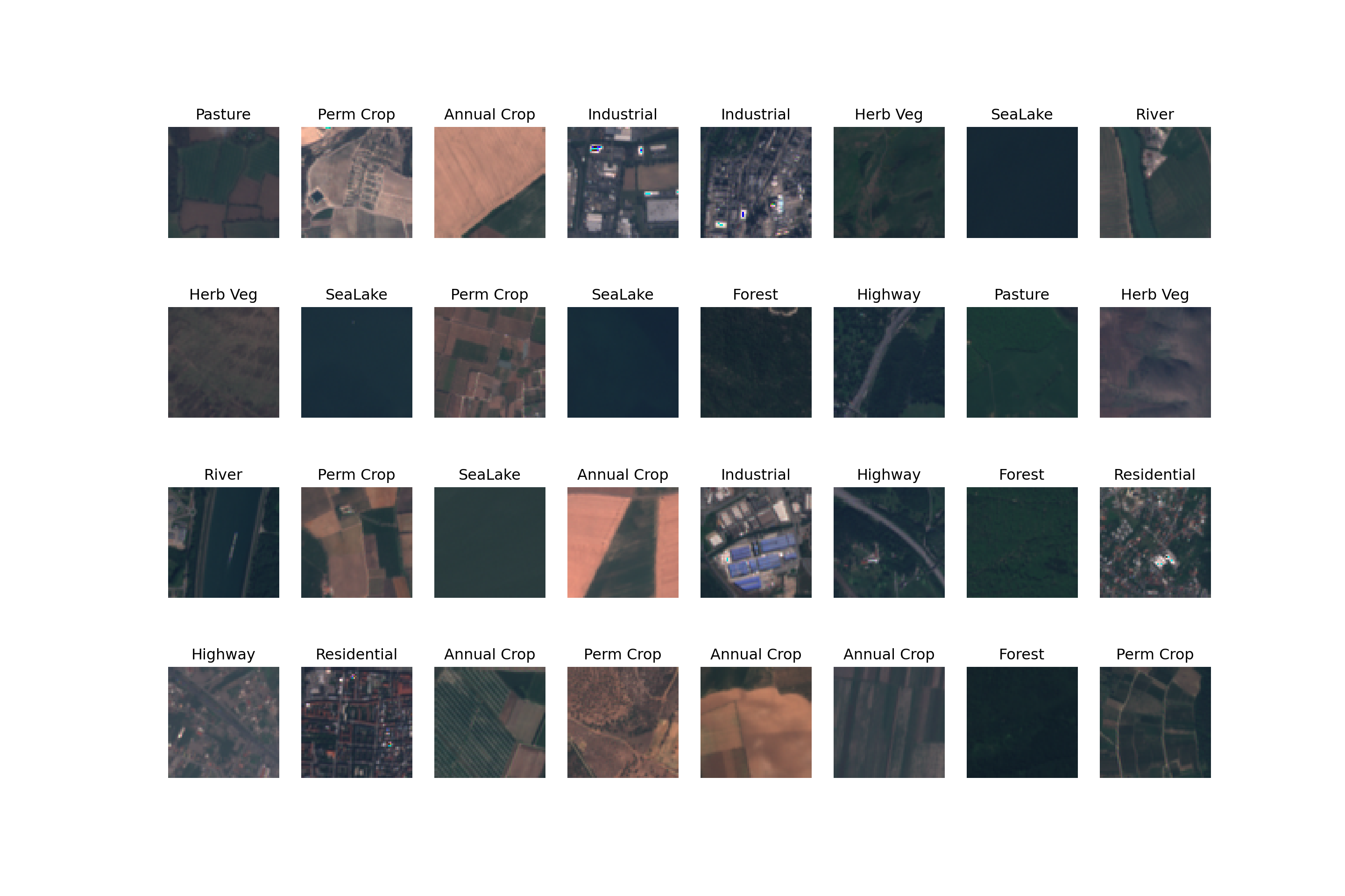

Define CNN Achitecture

As normal, I define the neural network architecture by subclassing nn.Module. This is the same architecture as was created in the prior module. A few reminders about how this is constructed.

The __init__() constructor method defines the parameters of the subclass. It accepts the number of classes to differentiate (inCls), input number of channels (inChn), number of output channels for each 2D convolution layer (outChn), number of nodes in the fully connected layers (fcChn), and the dimensions of the array after the last CNN max pooling operation is applied.
In the __init__() constructor method, I define the structure of the CNN. I have broken this into two components, each of which are defined within nn.Sequential(). The first component (cnnLyrs) defines the convolutional components while the second (fcLyrs) defines the fully connected layers.
The convolutional component of the architecture consists of the following:

2D Convolution –> Batch Normalization –> ReLU Activation –> Max Pooling –>

2D Convolution –> Batch Normalization–> ReLU Activation –> Max Pooling –>

2D Convolution –> Batch Normalization –> ReLU Activation –> Max Pooling

So, there are 4 sequences of 2D Convolution, batch normalization, ReLU activation, and max pooling. In each nn.Conv2d() layer, the kernel size is (3,3), the step size is 1, and the padding is 1. This results in no reduction in the spatial dimensions of the array. The nn.MaxPool2d() layers all use a kernel size of (2,2) and a stride of 2, which will result in reducing the size of the array by half in the spatial dimensions. In this case, the sequence will be:

(64,64) –> (32,32) –> (16,16) –> (8,8) –> (4,4)

Only the nn.Conv2d() and nn.BatchNorm2d() layers have trainable parameters in this component of the model.

In the fully connected component of the model, the sequence is as follows:

Fully Connected –> Batch Normalization –> ReLU Activation –> Fully Connected –> Batch Normalization –> ReLU Activation –> Fully Connected

The last fully connected layer is not followed by batch normalization and a ReLU activation since I want to output the class logits. I do not apply a softmax activation here since the loss function expects logits. The last nn.Linear() layer has an output size equal to the number of classes being differentiated. Also, I am using nn.BatchNorm1d() here as opposed to nn.BatchNorm2d() since I am now dealing with fully connected layers. Only the nn.Linear() and nn.BatchNorm1d() layers have trainable parameters in this component of the model.

The forward() method defines how data will pass through the network. It will first pass through the convolutional component, then be flattened, then pass through the fully connected layers. The flattening is accomplished using the view() method.

class myCNNSeq(nn.Module):
  def __init__(self, nCls, inChn, outChn, fcChn, lastDim):
    super().__init__()
    self.nCls = nCls
    self.inChn = inChn
    self.outChn = outChn
    self.fcChn = fcChn
    self.lastDim = lastDim

    self.cnnLyrs = nn.Sequential(
        nn.Conv2d(in_channels=inChn, out_channels=outChn[0], kernel_size=(3,3), padding=1),
        nn.BatchNorm2d(outChn[0]),
        nn.ReLU(inplace=True),
        nn.MaxPool2d(2,2),
        nn.Conv2d(in_channels=outChn[0], out_channels=outChn[1], kernel_size=(3,3), padding=1),
        nn.BatchNorm2d(outChn[1]),
        nn.ReLU(inplace=True),
        nn.MaxPool2d(2,2),
        nn.Conv2d(in_channels=outChn[1], out_channels=outChn[2], kernel_size=(3,3), padding=1),
        nn.BatchNorm2d(outChn[2]),
        nn.ReLU(inplace=True),
        nn.MaxPool2d(2,2),
        nn.Conv2d(in_channels=outChn[2], out_channels=outChn[3], kernel_size=(3,3), padding=1),
        nn.BatchNorm2d(outChn[3]),
        nn.ReLU(inplace=True),
        nn.MaxPool2d(2,2)   
    )

    self.fcLyrs = nn.Sequential(
        nn.Linear(lastDim*lastDim*outChn[3], fcChn[0]),
        nn.BatchNorm1d(fcChn[0]),
        nn.ReLU(inplace=True),
        nn.Linear(fcChn[0], fcChn[1]),
        nn.BatchNorm1d(fcChn[1]),
        nn.ReLU(inplace=True),
        nn.Linear(fcChn[1], nCls)
    )   
  
  def forward(self,x):
    x = self.cnnLyrs(x)
    x = x.view(-1, self.lastDim*self.lastDim*self.outChn[3])
    x = self.fcLyrs(x)
    return x

The getDim() function allows for determining the size of the array in the spatial dimensions for a given input size and for a given number of max pooling operations. This is used to determine the size of the array that will be flattened then provided as input to the fully connected component of the architecture.

def getDim(inDim, numBlks):
  x = inDim
  for i in range(1,numBlks+1,1):
    x = x/2
  return int(x)

I now instantiate an instance of the CNN. For this problem, the number of classes is 10 and the number of input channels is 10. I have set the output sizes, or number of learned kernels, to [10, 20, 30, 40]. This argument is provided as a list. The number of nodes in the fully connected layers are 256 and 512. Lastly, the size of the array at the end of the convolutional operations and prior to being flattened and fed into the fully connected component is calculated using the getDim() function, which accepts the original size of the image and the number of max pooling operations. Lastly, the model is moved to the device using the to() method.

model = myCNNSeq(nCls=10, 
                inChn=10, 
                outChn=[10,20,30,40],
                fcChn=[268,512],
                lastDim=getDim(64,4)).to(device)

Training Loop

Before training the model, I must define an optimizer and a loss metric. Here, I am using the AdamW optimizer, an augmented version of mini-batch gradient descent. It will optimize the trainable parameters associated with the model (model.parameters()). Since I do not set a learning rate, the default learning rate is used (0.001).

Since this is a multiclass classification problem, I am using cross entropy loss. The implementation of this loss in PyTorch expects logits as opposed to probabilities; this is why I did not include a softmax activation as the final step in the CNN architecture. This should be an adequate loss metric for this problem. This loss can sometimes perform poorly, especially if the classes are highly imbalanced, which is not the case here. If classes are highly imbalanced, it is possible to include class weights in the loss metric computation. Alternatively, a different loss can be used, such as DICE or Tversky loss. We will explore some of these options in the context of semantic segmentation. For now, we will stick with cross entropy loss.

optimizer = torch.optim.AdamW(model.parameters())

criterion = nn.CrossEntropyLoss().to(device)

In order to further monitor the training process and model performance, I define three assessment metrics, which are made available by the torchmetrics package. I will specifically calculate overall accuracy, class-aggregated F1-score, and the Kappa statistic.

The torchmetrics package has other parameters that can be specified for assessment metrics. For example, you can set a multidimensional averaging method that defines how dimensions are handled or reduced. Here, all dimensions are flattened, which is the default. You can also choose to ignore an index or class in the calculations. This is sometimes used if you have a “not labeled” or “missing” class that should not be considered. If you want to learn more about the torchmetrics package, please consult the associated documentation: https://torchmetrics.readthedocs.io/en/stable/.

acc = tm.Accuracy(task="multiclass", num_classes=10).to(device)
f1 = tm.F1Score(task="multiclass", num_classes=10).to(device)
kappa = tm.CohenKappa(task="multiclass", num_classes=10).to(device)

Lastly, I define the number of training epochs (50) and a folder in which to save the trained models.

epochs = 50
saveFolder = "C:/myFiles/work/dl/eurosat_cnn_models/"

I am now ready to train the model using a training loop. This loop is very similar to the loop used to train the fully connected neural network in the prior module. Let’s review the process. If you choose to run this code, it will take some time to execute. On my machine it took nearly 4 hours to train the network for 50 epochs. In contrast to the fully connected example, I am not saving the model to disk after each epoch. Instead, I write over a prior saved model if the performance improves. Specifically, if the current model provides a larger class-aggregated F1-score for predicting to the validation data, it will overwrite the prior model. This is accomplished by initializing a variable called f1VMax with a starting value of 0.0. At the end of each epoch, if the F1-score improves, this variable is updated to reflect that score and the model is saved. If the score does not improve, then the new model is not saved.

The steps below summarize the training loop.

I initialize a series of empty lists which will store the losses and assessment metrics calculated at each epoch. A total of 9 lists are created to store the epoch number (eNum), training loss (t_loss), training overall accuracy (t_acc), training F1-score (t_f1), training Kappa (t_kappa), validation loss (v_loss), validation accuracy (v_acc), validation F1-score (v_f1), and validation kappa (v_kappa). The f1VMax variable is initialized with a value of 0.0.
The training loop iterates over the number of epochs. This is the outer most for loop.
For the training data, it iterates over the batches as define by the DataLoader. I use enumerate() here since I need access to both the data and the associated index within the loop.
Within the training portion of the loop the following steps occur: (1) a batch is read in and moved to the device with the predictor variables (inputs) and labels (targets) stored in separate tensors; (2) the gradients are cleared so that each iteration of the loop acts as an independent weight update; (3) the model is applied to predict to the predictor variables (e.g., image pixels); (4) the loss is calculated using the predictions and labels; (5) the assessment metrics are calculated using the predictions and labels; (6) backpropagation is performed; and (7) an optimization step is performed to update the weights.
After one complete iteration over all of the training batches (i.e., one training epoch), the assessment metrics are accumulated across epochs; a result is printed consisting of the epoch number, the training loss, the training accuracy, the training class-aggregated F1-score, and the training Kappa. The epoch number, training loss, and accumulated assessment metrics are saved to the appropriate list objects. Since the accuracy, F1-score, and Kappa statistic are stored as tensors on the GPU, they must be detached, moved to the CPU, and converted to numpy arrays prior to being appended to the list.
At the end of each training epoch, the validation data are predicted in a separate loop over the validation batches. This occurs with the condition: with torch.no_grad(). This is so that the validation data predictions and loss calculations do not impact the gradients. Again, the model should not learn from the validation data, as this would be a data leak. In such a case, the validation data would not offer an unbiased assessment of model performance.
For each validation batch: (1) the predictor variables and targets are read and moved to the device; (2) the model is used to predict to the predictor variables; (3) the loss is calculated using the predictions and target labels; and (4) the assessment metrics are calculated.
Once all of the validation batches have been predicted: (1) the assessment metrics are accumulated across the batches; (2) a print statement is provided that includes the validation loss, validation accuracy, validation F1-score, and validation Kappa statistic; (3) the validation loss and assessment metrics are appended to the appropriate lists (again, the assessment metrics must be moved to the CPU and converted to numpy arrays prior to being appended); and (4) the validation assessment metrics are reset.
At the end of each epoch, an if statement is used to test whether the F1-score calculated using the validation data has improved. If it has, that value is saved to the f1VMax variable and the model is saved to disk. If not, then the f1VMax variable is not updated and the prior model saved to disk is not overwritten.

eNum = []
t_loss = []
t_acc = []
t_f1 = []
t_kappa = []
v_loss = []
v_acc = []
v_f1 = []
v_kappa = []

f1VMax = 0.0

# Loop over epochs
for epoch in range(1, epochs+1):
    # Loop over training batches
    for batch_idx, (inputs, targets) in enumerate(trainDL):
        # Get data and move to device
        inputs, targets = inputs.to(device), targets.to(device)

        # Clear gradients
        optimizer.zero_grad()
        # Predict data
        outputs = model(inputs)
        # Calculate loss
        loss = criterion(outputs, targets)

        # Calculate metrics
        accT = acc(outputs, targets)
        f1T = f1(outputs, targets)
        kappaT = kappa(outputs, targets)
        
        # Backpropagate
        loss.backward()

        # Update parameters
        optimizer.step()

    # Accumulate metrics at end of training epoch
    accT = acc.compute()
    f1T = f1.compute()
    kappaT = kappa.compute()

    # Print Losses and metrics at end of each training epoch   
    print(f'Epoch: {epoch}, Training Loss: {loss.item():.4f}, Training Accuracy: {accT:.4f}, Training F1: {f1T:.4f}, Training Kappa: {kappaT:.4f}')

    # Append results
    eNum.append(epoch)
    t_loss.append(loss.item())
    t_acc.append(accT.detach().cpu().numpy())
    t_f1.append(f1T.detach().cpu().numpy())
    t_kappa.append(kappaT.detach().cpu().numpy())

    # Reset metrics
    acc.reset()
    f1.reset()
    kappa.reset()

    # loop over validation batches
    with torch.no_grad():
        for batch_idx, (inputs, targets) in enumerate(valDL):
            # Get data and move to device
            inputs, targets = inputs.to(device), targets.to(device)

            # Predict data
            outputs = model(inputs)
            # Calculate validation loss
            loss_v = criterion(outputs, targets)

            # Calculate metrics
            accV = acc(outputs, targets)
            f1V = f1(outputs, targets)
            kappaV = kappa(outputs, targets)
            
    # Accumulate metrics at end of validation epoch
    accV = acc.compute()
    f1V = f1.compute()
    kappaV = kappa.compute()

    # Print validation loss and metrics
    print(f'Validation Loss: {loss_v.item():.4f}, Validation Accuracy: {accV:.4f}, Validation F1: {f1V:.4f}, Validation Kappa: {kappaV:.4f}')

    # Append results
    v_loss.append(loss_v.item())
    v_acc.append(accV.detach().cpu().numpy())
    v_f1.append(f1V.detach().cpu().numpy())
    v_kappa.append(kappaV.detach().cpu().numpy())

    # Reset metrics
    acc.reset()
    f1.reset()
    kappa.reset()

    # Save model if validation F1-score improves
    f1V2 = f1V.detach().cpu().numpy()
    if f1V2 > f1VMax:
        f1VMax = f1V2
        torch.save(model.state_dict(), saveFolder + 'eurosat_model.pt')
        print(f'Model saved for epoch {epoch}.')

Once the network is trained, we can explore the training process using the saved losses and assessment metrics. The code below is exactly the same as the code that was used to explore the fully connected neural network results from the prior module.

The model did not improve much after 30 epochs, suggesting that 50 epochs was long enough to train the model. The F1-scores suggest that the performance for the training data was still improving after 50 epochs. However, the results for the validation data leveled off after 30 epochs. Again, this suggests that 50 epochs was adequate to stabilize the results. The loss curves do not suggest overfitting. In short, the training process seems to have progressed smoothly. This was a fairly simple CNN, so it should not be expected that state-of-the-art performance would be obtained. However, the model did perform well in general. As noted in prior modules, if the performance was not adequate, I could experiment with altering the training process or model architecture. For example, I could use a different loss function, incorporate class weights or some other means to deal with data imbalance, incorporate dropouts, change the data augmentations applied, use a learning rate finder and/or learning rate scheduler, use a different optimization algorithm, and/or increase the number of convolutional layers and/or the number of learned kernels in each layer.

SeNum = pd.Series(eNum, name="epoch")
St_loss = pd.Series(t_loss, name="training_loss")
St_acc = pd.Series(t_acc, name="training_accuracy")
St_f1 = pd.Series(t_f1, name="training_f1")
St_kappa = pd.Series(t_kappa, name="training_kappa")
Sv_loss = pd.Series(v_loss, name="val_loss")
Sv_acc = pd.Series(v_acc, name="val_accuracy")
Sv_f1 = pd.Series(v_f1, name="val_f1")
Sv_kappa = pd.Series(t_kappa, name="val_kappa")
resultsDF = pd.concat([SeNum, St_loss, St_acc, St_f1, St_kappa, Sv_loss, Sv_acc, Sv_f1, Sv_kappa], axis=1)

resultsDF.to_csv(saveFolder+"resultsCNN.csv")

resultsDF = pd.read_csv(saveFolder+"resultsCNN.csv")

plt.rcParams['figure.figsize'] = [10, 10]
firstPlot = resultsDF.plot(x='epoch', y="training_loss")
resultsDF.plot(x='epoch', y="val_loss", ax=firstPlot)
plt.show()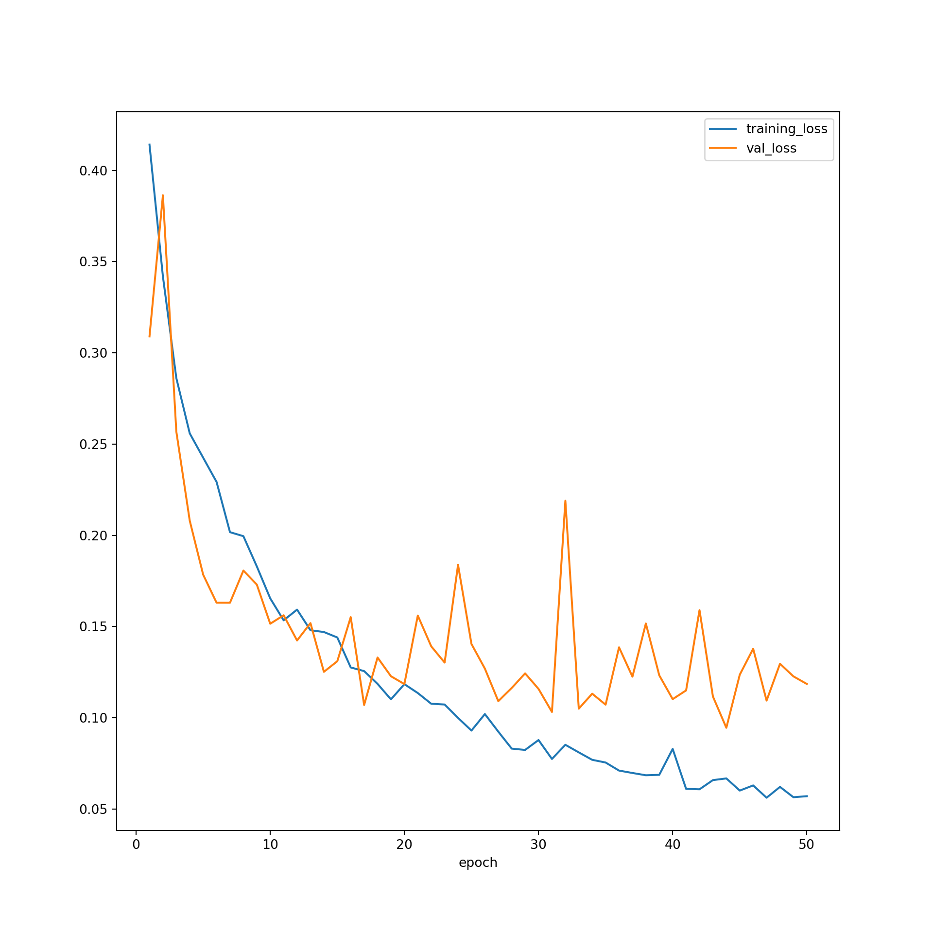

plt.rcParams['figure.figsize'] = [10, 10]
firstPlot = resultsDF.plot(x="epoch", y="training_f1")
resultsDF.plot(x='epoch', y="val_f1", ax=firstPlot)
plt.show()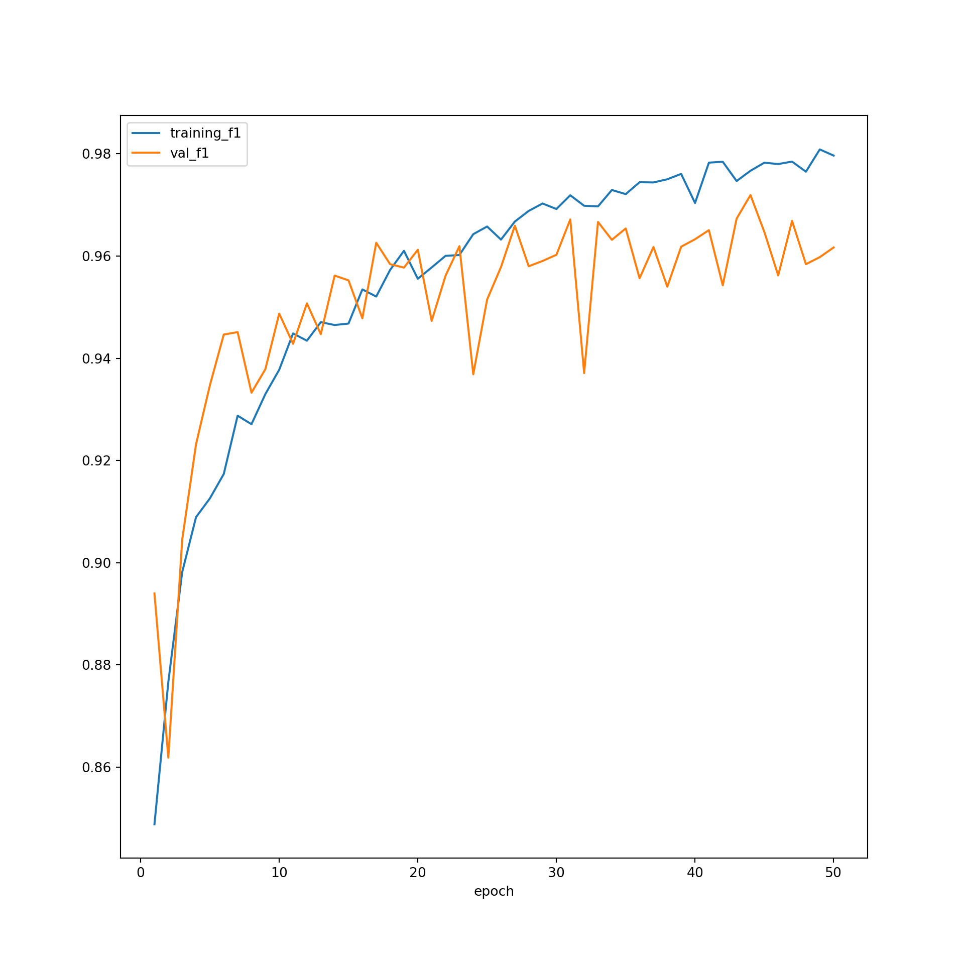

Assess Model

Lastly, I will predict to the withheld testing set. Before doing so, I re-instantiate the model and read in the saved weights from disk so that the best performing weights are used as opposed to the state after 50 epochs. In order to predict the test data, I have to (1) instantiate a new DataSet that references the testing DataFrame, (2) create a DataLoader from this DataSet, and (3) predict the new data with the trained model. The assessment metrics are accumulated over the batches using the compute() method from torchmetrics.

In comparison to our fully connected model, I am generally seeing stronger performance. I achieve an overall accuracy of around 98.7%. Again, this is not state-of-the-art performance, but is still pretty good.

model = myCNNSeq(nCls=10, 
                inChn=10, 
                outChn=[10,20,30,40],
                fcChn=[268,512],
                lastDim=getDim(64,4)).to(device)

saveFolder = "C:/myFiles/work/dl/eurosat_cnn_models/"
best_weights = torch.load(saveFolder+'eurosat_cnn_model.pt')
model.load_state_dict(best_weights)

<All keys matched successfully>

testDS = EuroSat(test, mnImg, sdImg, transform=None)

testDL = torch.utils.data.DataLoader(testDS, batch_size=32, shuffle=False, sampler=None,
num_workers=0, pin_memory=False, drop_last=True)

model.eval()

myCNNSeq(
  (cnnLyrs): Sequential(
    (0): Conv2d(10, 10, kernel_size=(3, 3), stride=(1, 1), padding=(1, 1))
    (1): BatchNorm2d(10, eps=1e-05, momentum=0.1, affine=True, track_running_stats=True)
    (2): ReLU(inplace=True)
    (3): MaxPool2d(kernel_size=2, stride=2, padding=0, dilation=1, ceil_mode=False)
    (4): Conv2d(10, 20, kernel_size=(3, 3), stride=(1, 1), padding=(1, 1))
    (5): BatchNorm2d(20, eps=1e-05, momentum=0.1, affine=True, track_running_stats=True)
    (6): ReLU(inplace=True)
    (7): MaxPool2d(kernel_size=2, stride=2, padding=0, dilation=1, ceil_mode=False)
    (8): Conv2d(20, 30, kernel_size=(3, 3), stride=(1, 1), padding=(1, 1))
    (9): BatchNorm2d(30, eps=1e-05, momentum=0.1, affine=True, track_running_stats=True)
    (10): ReLU(inplace=True)
    (11): MaxPool2d(kernel_size=2, stride=2, padding=0, dilation=1, ceil_mode=False)
    (12): Conv2d(30, 40, kernel_size=(3, 3), stride=(1, 1), padding=(1, 1))
    (13): BatchNorm2d(40, eps=1e-05, momentum=0.1, affine=True, track_running_stats=True)
    (14): ReLU(inplace=True)
    (15): MaxPool2d(kernel_size=2, stride=2, padding=0, dilation=1, ceil_mode=False)
  )
  (fcLyrs): Sequential(
    (0): Linear(in_features=640, out_features=268, bias=True)
    (1): BatchNorm1d(268, eps=1e-05, momentum=0.1, affine=True, track_running_stats=True)
    (2): ReLU(inplace=True)
    (3): Linear(in_features=268, out_features=512, bias=True)
    (4): BatchNorm1d(512, eps=1e-05, momentum=0.1, affine=True, track_running_stats=True)
    (5): ReLU(inplace=True)
    (6): Linear(in_features=512, out_features=10, bias=True)
  )
)

with torch.no_grad():
    for batch_idx, (inputs, targets) in enumerate(testDL):
        inputs, targets = inputs.to(device), targets.to(device)
        outputs = model(inputs)
        loss_v = criterion(outputs, targets)
        accV = acc(outputs, targets)
        f1V = f1(outputs, targets)
        kappaV = kappa(outputs, targets)
accV = acc.compute()
f1V = f1.compute()
kappaV = kappa.compute()
acc.reset()
f1.reset()
kappa.reset()

print(accV)

tensor(0.9866, device='cuda:0')

print(f1V)

tensor(0.9866, device='cuda:0')

print(kappaV)

tensor(0.9850, device='cuda:0')

print(loss_v.item())

4.134376649744809e-05

It is also possible to obtain class-level metrics by setting the average parameter to “none”. Below I have obtained the full confusion matrix and the class-level F1-score, precision, and recall metrics using torchmetrics, the withheld testing data, and a validation loop.

cm = tm.ConfusionMatrix(task="multiclass", num_classes=10).to(device)
f1 = tm.F1Score(task="multiclass", num_classes=10, average="none").to(device)
recall = tm.Precision(task="multiclass", num_classes=10, average="none").to(device)
precision = tm.Recall(task="multiclass", num_classes=10, average="none").to(device)

model.eval()

myCNNSeq(
  (cnnLyrs): Sequential(
    (0): Conv2d(10, 10, kernel_size=(3, 3), stride=(1, 1), padding=(1, 1))
    (1): BatchNorm2d(10, eps=1e-05, momentum=0.1, affine=True, track_running_stats=True)
    (2): ReLU(inplace=True)
    (3): MaxPool2d(kernel_size=2, stride=2, padding=0, dilation=1, ceil_mode=False)
    (4): Conv2d(10, 20, kernel_size=(3, 3), stride=(1, 1), padding=(1, 1))
    (5): BatchNorm2d(20, eps=1e-05, momentum=0.1, affine=True, track_running_stats=True)
    (6): ReLU(inplace=True)
    (7): MaxPool2d(kernel_size=2, stride=2, padding=0, dilation=1, ceil_mode=False)
    (8): Conv2d(20, 30, kernel_size=(3, 3), stride=(1, 1), padding=(1, 1))
    (9): BatchNorm2d(30, eps=1e-05, momentum=0.1, affine=True, track_running_stats=True)
    (10): ReLU(inplace=True)
    (11): MaxPool2d(kernel_size=2, stride=2, padding=0, dilation=1, ceil_mode=False)
    (12): Conv2d(30, 40, kernel_size=(3, 3), stride=(1, 1), padding=(1, 1))
    (13): BatchNorm2d(40, eps=1e-05, momentum=0.1, affine=True, track_running_stats=True)
    (14): ReLU(inplace=True)
    (15): MaxPool2d(kernel_size=2, stride=2, padding=0, dilation=1, ceil_mode=False)
  )
  (fcLyrs): Sequential(
    (0): Linear(in_features=640, out_features=268, bias=True)
    (1): BatchNorm1d(268, eps=1e-05, momentum=0.1, affine=True, track_running_stats=True)
    (2): ReLU(inplace=True)
    (3): Linear(in_features=268, out_features=512, bias=True)
    (4): BatchNorm1d(512, eps=1e-05, momentum=0.1, affine=True, track_running_stats=True)
    (5): ReLU(inplace=True)
    (6): Linear(in_features=512, out_features=10, bias=True)
  )
)

with torch.no_grad():
    for batch_idx, (inputs, targets) in enumerate(testDL):
        inputs, targets = inputs.to(device), targets.to(device)
        outputs = model(inputs)
        cmV = cm(outputs, targets)
        f1V = f1(outputs, targets)
        pV = precision(outputs, targets)
        rV = recall(outputs, targets)
cmV =cm.compute()
f1V = f1.compute()
pV = precision.compute()
rV = recall.compute()
cm.reset()
f1.reset()
precision.reset()
recall.reset()

print(cmV)

tensor([[591,   3,   1,   0,   0,   2,   1,   0,   2,   0],
        [  0, 598,   1,   0,   0,   1,   0,   0,   0,   0],
        [  1,   4, 590,   0,   0,   1,   3,   1,   0,   0],
        [  1,   0,   0, 486,   2,   3,   2,   1,   5,   0],
        [  0,   0,   0,   0, 495,   0,   0,   4,   1,   0],
        [  2,   2,   4,   0,   0, 385,   6,   0,   1,   0],
        [  2,   0,   7,   0,   0,   1, 490,   0,   0,   0],
        [  0,   0,   0,   1,   3,   0,   0, 596,   0,   0],
        [  0,   0,   1,   0,   1,   2,   0,   0, 496,   0],
        [  0,   0,   0,   0,   0,   0,   0,   0,   1, 703]], device='cuda:0')

print(f1V)

tensor([0.9875, 0.9909, 0.9801, 0.9848, 0.9890, 0.9686, 0.9780, 0.9917, 0.9861,
        0.9993], device='cuda:0')

print(pV)

tensor([0.9850, 0.9967, 0.9833, 0.9720, 0.9900, 0.9625, 0.9800, 0.9933, 0.9920,
        0.9986], device='cuda:0')

print(rV)

tensor([0.9899, 0.9852, 0.9768, 0.9979, 0.9880, 0.9747, 0.9761, 0.9900, 0.9802,
        1.0000], device='cuda:0')

Concluding Remarks

The goal of this module was to demonstrate the process of training and assessing a CNN for scene classification or scene labeling tasks. Before moving on to discuss pixel-level classification, or semantic segmentation, in the next module we will explore some famous and powerful CNN architectures, specifically VGGNet and ResNet, which can be easily implemented using torchvision.