Train UNet
Train a UNet for Semantic Segmentation
Introduction
Now that we have covered building a UNet semantic segmentation architecture, we are ready to use it to make predictions at the pixel-level. Fortunately, you will see that the training and validation processes are very similar to the processes we have already explored for fully connected and convolutional neural networks for scene labeling.
As usual, I begin by reading in the needed libraries including numpy, pandas, matplotlib, os, and torch. In this example, I will use the OpenCV package (cv2) (https://pypi.org/project/opencv-python/) to read in the image data. I will use the albumentations package (https://albumentations.ai/) to apply data augmentations, as I have found it to be better for semantic segmentation tasks in comparison to using the transformations available in torchvision. This is because the package does a good job of augmenting the pixel-level labels along with the image chips. For example, if the image is flipped, the mask will also be flipped to maintain alignment. I use torchinfo to obtain a summary of the architecture and torchmetrics to calculate assessment metrics. Lastly, the segmentation models library (https://github.com/qubvel/segmentation_models.pytorch) is used to implement a multi-class Dice loss. We will explore this package in more detail in a later module. Here, I am just using a loss metric that it provides.
I run this experiment on a GPU. This process could not be implemented on a CPU, as it is too computationally intensive. I have provided a trained model if you do not want to or cannot execute the training loop on your machine.
import numpy as np
import pandas as pd
import matplotlib
from matplotlib import pyplot as plt

import os

import cv2

import albumentations as A

import torch
import torch.nn as nn
from torch.nn import functional as F
from torch.utils.data.dataset import Dataset
from torch.utils.data import DataLoader

from torchinfo import summary

import torchmetrics as tm

from kornia import losses
device = torch.device("cuda:0" if torch.cuda.is_available() else "cpu")
print(device)cuda:0In this example, I will attempt to build a model to classify general land cover classes from true color, or RGB, aerial orthophotography using the Landcover.ai dataset. This dataset consists of 41 orthophotos with a spatial resolution of between 25 and 50 cm for areas in Poland. Five classes are differentiated:
0 = Other
1 = Building
2 = Woodland
3 = Water
4 = Road
These data are introduced and described in the following publication and can be downloaded at https://landcover.ai.linuxpolska.com/.
Boguszewski, A., Batorski, D., Ziemba-Jankowska, N., Dziedzic, T. and Zambrzycka, A., 2021. LandCover. ai: Dataset for automatic mapping of buildings, woodlands, water and roads from aerial imagery. In Proceedings of the IEEE/CVF Conference on Computer Vision and Pattern Recognition (pp. 1102-1110).
Preparation
Before using these data, the provided orthophotos must be partitioned into smaller image and associated mask chips. The data originators have provided a script to accomplish this task that is included with the data download. You will need to change the IMGS_DIR, MASK_DIR, and OUTPUT_DIR directories to the correct path on your machine. The OUTPUT_DIR directory will be created as part of the execution. This script generates chips with a 512x512 pixel size. The produced chips will match the file names provided in the provided train.txt, val.txt, and test.txt files that are also provided with the data. I have commented this code out in the example since I have already generated the chips. However, you will need to run it in order to generate the image chips on your local machine. Note that we will explore generating our own image chips in a later module.
"""
import glob
import os

import cv2

IMGS_DIR = "C:/myFiles/work/dl/landcover.ai.v1/images/"
MASKS_DIR = "C:/myFiles/work/dl/landcover.ai.v1/masks/"
OUTPUT_DIR = "C:/myFiles/work/dl/lancoverai/"

TARGET_SIZE = 512

img_paths = glob.glob(os.path.join(IMGS_DIR, "*.tif"))
mask_paths = glob.glob(os.path.join(MASKS_DIR, "*.tif"))

img_paths.sort()
mask_paths.sort()

os.makedirs(OUTPUT_DIR)
for i, (img_path, mask_path) in enumerate(zip(img_paths, mask_paths)):
    img_filename = os.path.splitext(os.path.basename(img_path))[0]
    mask_filename = os.path.splitext(os.path.basename(mask_path))[0]
    img = cv2.imread(img_path)
    mask = cv2.imread(mask_path)

    assert img_filename == mask_filename and img.shape[:2] == mask.shape[:2]

    k = 0
    for y in range(0, img.shape[0], TARGET_SIZE):
        for x in range(0, img.shape[1], TARGET_SIZE):
            img_tile = img[y:y + TARGET_SIZE, x:x + TARGET_SIZE]
            mask_tile = mask[y:y + TARGET_SIZE, x:x + TARGET_SIZE]

            if img_tile.shape[0] == TARGET_SIZE and img_tile.shape[1] == TARGET_SIZE:
                out_img_path = os.path.join(OUTPUT_DIR, "{}_{}.jpg".format(img_filename, k))
                cv2.imwrite(out_img_path, img_tile)

                out_mask_path = os.path.join(OUTPUT_DIR, "{}_{}_m.png".format(mask_filename, k))
                cv2.imwrite(out_mask_path, mask_tile)

            k += 1

    print("Processed {} {}/{}".format(img_filename, i + 1, len(img_paths)))
"""
'\nimport glob\nimport os\n\nimport cv2\n\nIMGS_DIR = "C:/myFiles/work/dl/landcover.ai.v1/images/"\nMASKS_DIR = "C:/myFiles/work/dl/landcover.ai.v1/masks/"\nOUTPUT_DIR = "C:/myFiles/work/dl/lancoverai/"\n\nTARGET_SIZE = 512\n\nimg_paths = glob.glob(os.path.join(IMGS_DIR, "*.tif"))\nmask_paths = glob.glob(os.path.join(MASKS_DIR, "*.tif"))\n\nimg_paths.sort()\nmask_paths.sort()\n\nos.makedirs(OUTPUT_DIR)\nfor i, (img_path, mask_path) in enumerate(zip(img_paths, mask_paths)):\n img_filename = os.path.splitext(os.path.basename(img_path))[0]\n mask_filename = os.path.splitext(os.path.basename(mask_path))[0]\n img = cv2.imread(img_path)\n mask = cv2.imread(mask_path)\n\n assert img_filename == mask_filename and img.shape[:2] == mask.shape[:2]\n\n k = 0\n for y in range(0, img.shape[0], TARGET_SIZE):\n for x in range(0, img.shape[1], TARGET_SIZE):\n img_tile = img[y:y + TARGET_SIZE, x:x + TARGET_SIZE]\n mask_tile = mask[y:y + TARGET_SIZE, x:x + TARGET_SIZE]\n\n if img_tile.shape[0] == TARGET_SIZE and img_tile.shape[1] == TARGET_SIZE:\n out_img_path = os.path.join(OUTPUT_DIR, "{}_{}.jpg".format(img_filename, k))\n cv2.imwrite(out_img_path, img_tile)\n\n out_mask_path = os.path.join(OUTPUT_DIR, "{}_{}_m.png".format(mask_filename, k))\n cv2.imwrite(out_mask_path, mask_tile)\n\n k += 1\n\n print("Processed {} {}/{}".format(img_filename, i + 1, len(img_paths)))\n'I next continue the preparation work by (1) creating a list of the class names, (2) saving the string representing the path to the folder in which I want to save results to a variable, and (3) reading in the provided train.txt, val.txt, and test.txt tables as pandas DataFrames. I then add new “img” and “mask” columns to the data tables to store the full, local file path to the image chips and associated masks, respectively. Note that the images are stored in JPEG format while the masks are stored in PNG format.
CLASSES = ['background', 'building', 'woodlands', 'water', 'road']
OUTPUT_DIR = "C:/myFiles/work/dl/lancoverai/"
trainDF = pd.read_csv("C:/myFiles/work/dl/landcover.ai.v1/train.txt", header=None, names=["file"])
trainDF["img"] = OUTPUT_DIR + trainDF['file'] + ".jpg"
trainDF["mask"] = OUTPUT_DIR + trainDF['file'] + "_m.png"valDF = pd.read_csv("C:/myFiles/work/dl/landcover.ai.v1/val.txt", header=None, names=["file"])
valDF["img"] = OUTPUT_DIR + valDF['file'] + ".jpg"
valDF["mask"] = OUTPUT_DIR + valDF['file'] + "_m.png"testDF = pd.read_csv("C:/myFiles/work/dl/landcover.ai.v1/test.txt", header=None, names=["file"])
testDF["img"] = OUTPUT_DIR + testDF['file'] + ".jpg"
testDF["mask"] = OUTPUT_DIR + testDF['file'] + "_m.png"trainDF.head() file ... mask
0 M-33-20-D-c-4-2_0 ... C:/myFiles/work/dl/lancoverai/M-33-20-D-c-4-2_...
1 M-33-20-D-c-4-2_1 ... C:/myFiles/work/dl/lancoverai/M-33-20-D-c-4-2_...
2 M-33-20-D-c-4-2_10 ... C:/myFiles/work/dl/lancoverai/M-33-20-D-c-4-2_...
3 M-33-20-D-c-4-2_100 ... C:/myFiles/work/dl/lancoverai/M-33-20-D-c-4-2_...
4 M-33-20-D-c-4-2_102 ... C:/myFiles/work/dl/lancoverai/M-33-20-D-c-4-2_...
[5 rows x 3 columns]I next subclass the Dataset class to build a subclass to read the image chips and associated masks. The key components are described below.
- Accepts an input DataFrame and a transforms object, which will be defined below using albumentations.
- Reads in the image chips and masks with cv2. I also reorder the bands from BGR to RGB and convert the image to an unsigned 8-bit data type.
- Transforms are applied if they are defined, or if the transform parameter is not “None”. Transforms are applied to both the image and the associated mask (i.e., pixel-level labels).
- The images and masks are converted to tensors using the from_numpy() function.
- The image is converted to the channels-first convention. This is necessary because cv2 reads in data using the channels-last convention while PyTorch expects channels-first.
- The image data are converted to a float data type (32-bit) then divided by 255 to rescale the data from 0 to 255 to 0 to 1. This works because the original image digital number (DN) values are on an 8-bit radiometric scale.
- The image is converted to a long integer (64-bit) data type.
# Subclass and define custom dataset ===========================
class MultiClassSegDataset(Dataset):

    def __init__(self, df, transform=None,):
        self.df = df
        self.transform = transform

    def __getitem__(self, idx):

        image_name = self.df.iloc[idx, 1]
        mask_name = self.df.iloc[idx, 2]
        image = cv2.imread(image_name)
        image = cv2.cvtColor(image, cv2.COLOR_BGR2RGB)
        mask = cv2.imread(mask_name, cv2.IMREAD_UNCHANGED)
        image = image.astype('uint8')
        mask = mask[:,:,0]
        if(self.transform is not None):
            transformed = self.transform(image=image, mask=mask)
            image = transformed["image"]
            mask = transformed["mask"]
            image = torch.from_numpy(image)
            mask = torch.from_numpy(mask)
            image = image.permute(2, 0, 1)
            image = image.float()/255
            mask = mask.long()
        else:
            image = torch.from_numpy(image)
            mask = torch.from_numpy(mask)
            image = image.permute(2, 0, 1)
            image = image.float()/255
            mask = mask.long()
        return image, mask

    def __len__(self):
        return len(self.df)
Transforms are defined in the code blocks below using albumentations. For the validation and testing data, the only applied transform is to add padding and/or resize the data so that they have a size of 512x512 pixels. This is not strictly necessary since all data should already have these dimensions.
For the training data, I will apply additional random transformations as a form of data augmentation in an attempt to combat overfitting. These include random changes to brightness and/or contrast, horizontal flips, vertical flips, and median blurring. The p parameter controls the likelihood or probability of these random augmentation being applied. There are some additional specific arguments for some of the transformations. If you are interested in further exploring what augmentations can be applied and the associated settings, please consult the albumentations package documentation.
test_transform = A.Compose(
    [A.PadIfNeeded(min_height=512, min_width=512, border_mode=4), A.Resize(512, 512),]
)
train_transform = A.Compose(
[
A.PadIfNeeded(min_height=512, min_width=512, border_mode=4),
A.Resize(512, 512),
A.RandomBrightnessContrast(brightness_limit=0.3, contrast_limit=0.3, p=0.5),
A.HorizontalFlip(p=0.5),
A.VerticalFlip(p=0.5),
A.MedianBlur(blur_limit=3, always_apply=False, p=0.1),
]
)I next initialize the DataSets for both the training and validation data using the appropriate transformations. Printing the length of the datasets, you can see that there are 7,470 training chips and 1,602 validation chips.
The DataLoaders are then defined. I use a mini-batch size of 8; however, you may need to change this setting depending on your available GPU hardware. I shuffle the training data but not the validation data. For both cases, I drop the last mini-batch.
I next print information about the data mini-batches. The image mini-batches have a shape of (8, 3, 512, 512) and a data type of 32-bit float while the masks have a shape of (8, 512, 512) and a data type of long integer (64-bit). The mask data could be represented using a shape of (8, 1, 512, 512); however, the loss metric expects the image channel to not be included.
Printing information about a single image, you can see the image shape is (3, 512, 512) and the data type is 32-bit float. A single mask has a shape of (512, 512) and a data type of 64-bit integer (long).
Lastly, I use matplotlib and the imshow() function to plot an example image and mask. Note the need to permute the bands since matplotlib expects a channels-last as opposed to channels-first configuration.
trainDS = MultiClassSegDataset(trainDF, transform=train_transform)
valDS = MultiClassSegDataset(valDF, transform=test_transform)
print("Number of Training Samples: " + str(len(trainDS)) + " Number of Testing Samples: " + str(len(valDS)))
Number of Training Samples: 7470 Number of Testing Samples: 1602trainDL = DataLoader(trainDS, batch_size=8, shuffle=True, sampler=None,
batch_sampler=None, num_workers=0, collate_fn=None,
pin_memory=False, drop_last=True, timeout=0,
worker_init_fn=None)
valDL = DataLoader(valDS, batch_size=8, shuffle=False, sampler=None,
batch_sampler=None, num_workers=0, collate_fn=None,
pin_memory=False, drop_last=True, timeout=0,
worker_init_fn=None)batch = next(iter(trainDL))
images, labels = batch
print(images.shape, labels.shape, type(images), type(labels), images.dtype, labels.dtype)torch.Size([8, 3, 512, 512]) torch.Size([8, 512, 512]) <class 'torch.Tensor'> <class 'torch.Tensor'> torch.float32 torch.int64testImg = images[1]
testMsk = labels[1]
print(testImg.shape, testImg.dtype, type(testImg), testMsk.shape,
testMsk.dtype, type(testMsk), testImg.min(),
testImg.max(), testMsk.min(), testMsk.max())torch.Size([3, 512, 512]) torch.float32 <class 'torch.Tensor'> torch.Size([512, 512]) torch.int64 <class 'torch.Tensor'> tensor(0.1961) tensor(0.9608) tensor(0) tensor(2)# Plot example image =====================================
plt.imshow(testImg.permute(1,2,0))
plt.show()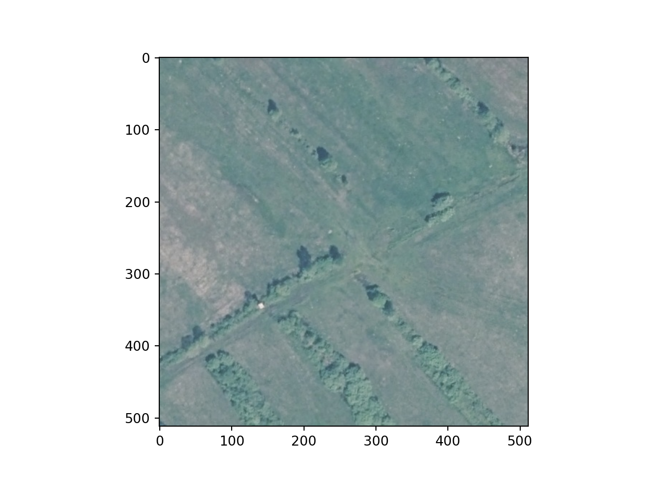
# Plot example image =====================================
plt.imshow(testMsk.unsqueeze(dim=0).permute(1,2,0))
plt.show()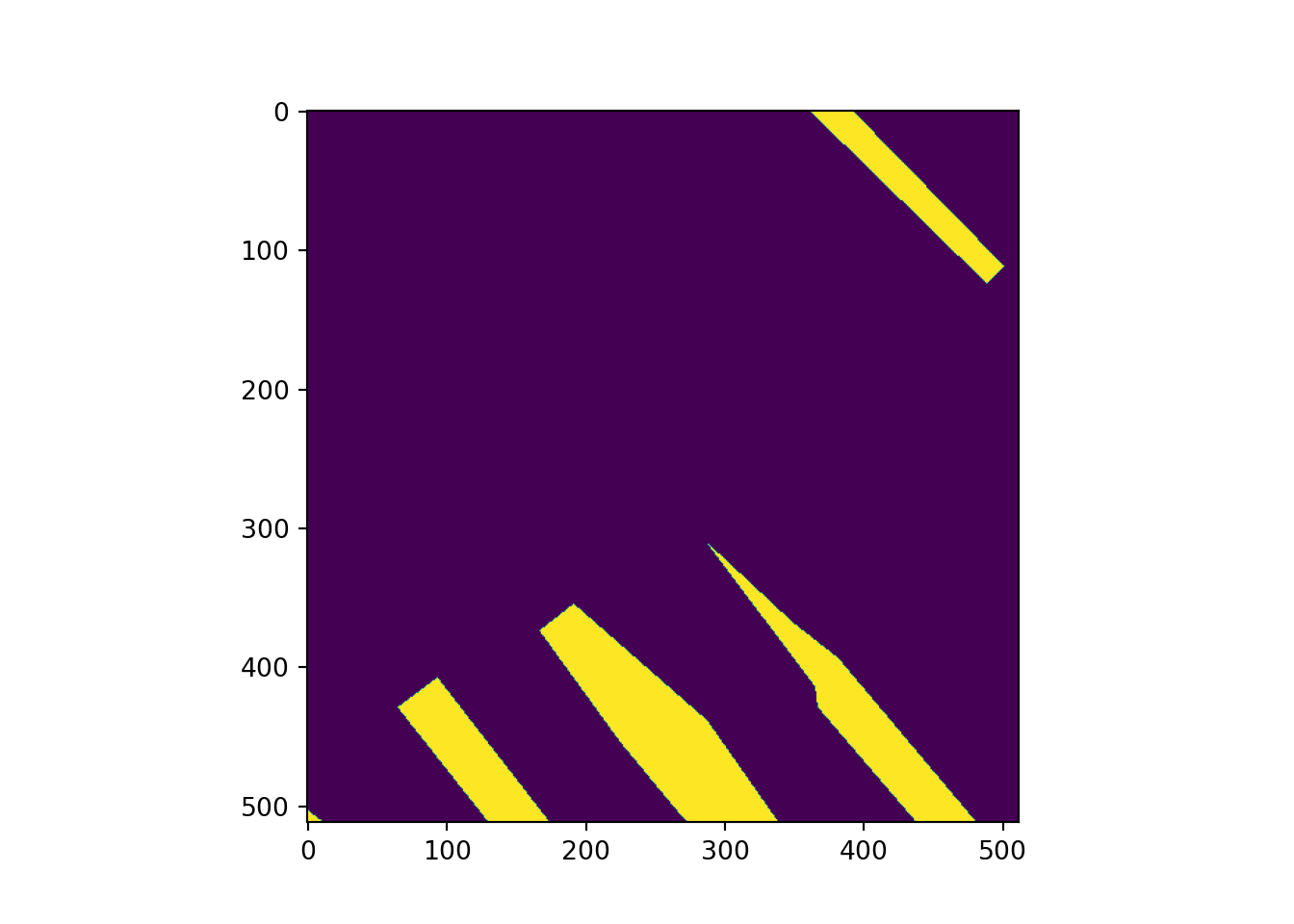
Define UNet
I next define the UNet architecture by subclassing nn.Module. This is the same architecture that was built in the last module, so we will not discuss the specifics here. Once the architecture is defined, I instantiate an instance that outputs 16, 32, 64, and 128 feature maps in the encoder blocks; 512 feature maps in the bottleneck block; and 128, 64, 32, and 16 feature maps in the decoder block. The architecture expects 3 input channels and differentiate 5 classes. Lastly, I print a summary of the model when provided the input shape being used here. This model has over 5 million trainable parameters.
def double_conv(inChannels, outChannels):
  return nn.Sequential(
      nn.Conv2d(inChannels, outChannels, kernel_size=(3,3), stride=1, padding=1),
      nn.BatchNorm2d(outChannels),
      nn.ReLU(inplace=True),
      nn.Conv2d(outChannels, outChannels, kernel_size=(3,3), stride=1, padding=1),
      nn.BatchNorm2d(outChannels),
      nn.ReLU(inplace=True)
  )
def up_conv(inChannels, outChannels):
return nn.Sequential(
nn.ConvTranspose2d(inChannels, outChannels, kernel_size=(2,2), stride=2),
nn.BatchNorm2d(outChannels),
nn.ReLU(inplace=True)
)class myUNet(nn.Module):
def __init__(self, encoderChn, decoderChn, inChn, botChn, nCls):
super().__init__()
self.encoderChn = encoderChn
self.decoderChn = decoderChn
self.botChn = botChn
self.nCls = nCls
self.encoder1 = double_conv(inChn, encoderChn[0])
self.encoder2 = nn.Sequential(nn.MaxPool2d(kernel_size=2, stride=2),
double_conv(encoderChn[0], encoderChn[1]))
self.encoder3 = nn.Sequential(nn.MaxPool2d(kernel_size=2, stride=2),
double_conv(encoderChn[1], encoderChn[2]))
self.encoder4 = nn.Sequential(nn.MaxPool2d(kernel_size=2, stride=2),
double_conv(encoderChn[2], encoderChn[3]))
self.bottleneck = nn.Sequential(nn.MaxPool2d(kernel_size=2, stride=2),
double_conv(encoderChn[3], botChn))
self.decoder1up = up_conv(botChn, botChn)
self.decoder1 = double_conv(encoderChn[3]+botChn, decoderChn[0])
self.decoder2up = up_conv(decoderChn[0], decoderChn[0])
self.decoder2 = double_conv(encoderChn[2]+decoderChn[0], decoderChn[1])
self.decoder3up = up_conv(decoderChn[1], decoderChn[1])
self.decoder3 = double_conv(encoderChn[1]+decoderChn[1], decoderChn[2])
self.decoder4up = up_conv(decoderChn[2], decoderChn[2])
self.decoder4 = double_conv(encoderChn[0]+decoderChn[2], decoderChn[3])
self.classifier = nn.Conv2d(decoderChn[3], nCls, kernel_size=(1,1))
def forward(self, x):
#Encoder
encoder1 = self.encoder1(x)
encoder2 = self.encoder2(encoder1)
encoder3 = self.encoder3(encoder2)
encoder4 = self.encoder4(encoder3)
#Bottleneck
x = self.bottleneck(encoder4)
#Decoder
x = self.decoder1up(x)
x = torch.concat([x, encoder4], dim=1)
x = self.decoder1(x)
x = self.decoder2up(x)
x = torch.concat([x, encoder3], dim=1)
x = self.decoder2(x)
x = self.decoder3up(x)
x = torch.concat([x, encoder2], dim=1)
x = self.decoder3(x)
x = self.decoder4up(x)
x = torch.concat([x, encoder1], dim=1)
x = self.decoder4(x)
#Classifier head
x = self.classifier(x)
return xmodel = myUNet(encoderChn=[16,32,64,128], decoderChn=[128,64,32,16], inChn=3, botChn=512, nCls=5).to(device)summary(model, (8, 3,512,512))==========================================================================================
Layer (type:depth-idx) Output Shape Param #
==========================================================================================
myUNet [8, 5, 512, 512] --
├─Sequential: 1-1 [8, 16, 512, 512] --
│ └─Conv2d: 2-1 [8, 16, 512, 512] 448
│ └─BatchNorm2d: 2-2 [8, 16, 512, 512] 32
│ └─ReLU: 2-3 [8, 16, 512, 512] --
│ └─Conv2d: 2-4 [8, 16, 512, 512] 2,320
│ └─BatchNorm2d: 2-5 [8, 16, 512, 512] 32
│ └─ReLU: 2-6 [8, 16, 512, 512] --
├─Sequential: 1-2 [8, 32, 256, 256] --
│ └─MaxPool2d: 2-7 [8, 16, 256, 256] --
│ └─Sequential: 2-8 [8, 32, 256, 256] --
│ │ └─Conv2d: 3-1 [8, 32, 256, 256] 4,640
│ │ └─BatchNorm2d: 3-2 [8, 32, 256, 256] 64
│ │ └─ReLU: 3-3 [8, 32, 256, 256] --
│ │ └─Conv2d: 3-4 [8, 32, 256, 256] 9,248
│ │ └─BatchNorm2d: 3-5 [8, 32, 256, 256] 64
│ │ └─ReLU: 3-6 [8, 32, 256, 256] --
├─Sequential: 1-3 [8, 64, 128, 128] --
│ └─MaxPool2d: 2-9 [8, 32, 128, 128] --
│ └─Sequential: 2-10 [8, 64, 128, 128] --
│ │ └─Conv2d: 3-7 [8, 64, 128, 128] 18,496
│ │ └─BatchNorm2d: 3-8 [8, 64, 128, 128] 128
│ │ └─ReLU: 3-9 [8, 64, 128, 128] --
│ │ └─Conv2d: 3-10 [8, 64, 128, 128] 36,928
│ │ └─BatchNorm2d: 3-11 [8, 64, 128, 128] 128
│ │ └─ReLU: 3-12 [8, 64, 128, 128] --
├─Sequential: 1-4 [8, 128, 64, 64] --
│ └─MaxPool2d: 2-11 [8, 64, 64, 64] --
│ └─Sequential: 2-12 [8, 128, 64, 64] --
│ │ └─Conv2d: 3-13 [8, 128, 64, 64] 73,856
│ │ └─BatchNorm2d: 3-14 [8, 128, 64, 64] 256
│ │ └─ReLU: 3-15 [8, 128, 64, 64] --
│ │ └─Conv2d: 3-16 [8, 128, 64, 64] 147,584
│ │ └─BatchNorm2d: 3-17 [8, 128, 64, 64] 256
│ │ └─ReLU: 3-18 [8, 128, 64, 64] --
├─Sequential: 1-5 [8, 512, 32, 32] --
│ └─MaxPool2d: 2-13 [8, 128, 32, 32] --
│ └─Sequential: 2-14 [8, 512, 32, 32] --
│ │ └─Conv2d: 3-19 [8, 512, 32, 32] 590,336
│ │ └─BatchNorm2d: 3-20 [8, 512, 32, 32] 1,024
│ │ └─ReLU: 3-21 [8, 512, 32, 32] --
│ │ └─Conv2d: 3-22 [8, 512, 32, 32] 2,359,808
│ │ └─BatchNorm2d: 3-23 [8, 512, 32, 32] 1,024
│ │ └─ReLU: 3-24 [8, 512, 32, 32] --
├─Sequential: 1-6 [8, 512, 64, 64] --
│ └─ConvTranspose2d: 2-15 [8, 512, 64, 64] 1,049,088
│ └─BatchNorm2d: 2-16 [8, 512, 64, 64] 1,024
│ └─ReLU: 2-17 [8, 512, 64, 64] --
├─Sequential: 1-7 [8, 128, 64, 64] --
│ └─Conv2d: 2-18 [8, 128, 64, 64] 737,408
│ └─BatchNorm2d: 2-19 [8, 128, 64, 64] 256
│ └─ReLU: 2-20 [8, 128, 64, 64] --
│ └─Conv2d: 2-21 [8, 128, 64, 64] 147,584
│ └─BatchNorm2d: 2-22 [8, 128, 64, 64] 256
│ └─ReLU: 2-23 [8, 128, 64, 64] --
├─Sequential: 1-8 [8, 128, 128, 128] --
│ └─ConvTranspose2d: 2-24 [8, 128, 128, 128] 65,664
│ └─BatchNorm2d: 2-25 [8, 128, 128, 128] 256
│ └─ReLU: 2-26 [8, 128, 128, 128] --
├─Sequential: 1-9 [8, 64, 128, 128] --
│ └─Conv2d: 2-27 [8, 64, 128, 128] 110,656
│ └─BatchNorm2d: 2-28 [8, 64, 128, 128] 128
│ └─ReLU: 2-29 [8, 64, 128, 128] --
│ └─Conv2d: 2-30 [8, 64, 128, 128] 36,928
│ └─BatchNorm2d: 2-31 [8, 64, 128, 128] 128
│ └─ReLU: 2-32 [8, 64, 128, 128] --
├─Sequential: 1-10 [8, 64, 256, 256] --
│ └─ConvTranspose2d: 2-33 [8, 64, 256, 256] 16,448
│ └─BatchNorm2d: 2-34 [8, 64, 256, 256] 128
│ └─ReLU: 2-35 [8, 64, 256, 256] --
├─Sequential: 1-11 [8, 32, 256, 256] --
│ └─Conv2d: 2-36 [8, 32, 256, 256] 27,680
│ └─BatchNorm2d: 2-37 [8, 32, 256, 256] 64
│ └─ReLU: 2-38 [8, 32, 256, 256] --
│ └─Conv2d: 2-39 [8, 32, 256, 256] 9,248
│ └─BatchNorm2d: 2-40 [8, 32, 256, 256] 64
│ └─ReLU: 2-41 [8, 32, 256, 256] --
├─Sequential: 1-12 [8, 32, 512, 512] --
│ └─ConvTranspose2d: 2-42 [8, 32, 512, 512] 4,128
│ └─BatchNorm2d: 2-43 [8, 32, 512, 512] 64
│ └─ReLU: 2-44 [8, 32, 512, 512] --
├─Sequential: 1-13 [8, 16, 512, 512] --
│ └─Conv2d: 2-45 [8, 16, 512, 512] 6,928
│ └─BatchNorm2d: 2-46 [8, 16, 512, 512] 32
│ └─ReLU: 2-47 [8, 16, 512, 512] --
│ └─Conv2d: 2-48 [8, 16, 512, 512] 2,320
│ └─BatchNorm2d: 2-49 [8, 16, 512, 512] 32
│ └─ReLU: 2-50 [8, 16, 512, 512] --
├─Conv2d: 1-14 [8, 5, 512, 512] 85
==========================================================================================
Total params: 5,463,269
Trainable params: 5,463,269
Non-trainable params: 0
Total mult-adds (G): 199.32
==========================================================================================
Input size (MB): 25.17
Forward/backward pass size (MB): 6392.12
Params size (MB): 21.85
Estimated Total Size (MB): 6439.14
==========================================================================================
==========================================================================================
Layer (type:depth-idx) Output Shape Param #
==========================================================================================
myUNet [8, 5, 512, 512] --
├─Sequential: 1-1 [8, 16, 512, 512] --
│ └─Conv2d: 2-1 [8, 16, 512, 512] 448
│ └─BatchNorm2d: 2-2 [8, 16, 512, 512] 32
│ └─ReLU: 2-3 [8, 16, 512, 512] --
│ └─Conv2d: 2-4 [8, 16, 512, 512] 2,320
│ └─BatchNorm2d: 2-5 [8, 16, 512, 512] 32
│ └─ReLU: 2-6 [8, 16, 512, 512] --
├─Sequential: 1-2 [8, 32, 256, 256] --
│ └─MaxPool2d: 2-7 [8, 16, 256, 256] --
│ └─Sequential: 2-8 [8, 32, 256, 256] --
│ │ └─Conv2d: 3-1 [8, 32, 256, 256] 4,640
│ │ └─BatchNorm2d: 3-2 [8, 32, 256, 256] 64
│ │ └─ReLU: 3-3 [8, 32, 256, 256] --
│ │ └─Conv2d: 3-4 [8, 32, 256, 256] 9,248
│ │ └─BatchNorm2d: 3-5 [8, 32, 256, 256] 64
│ │ └─ReLU: 3-6 [8, 32, 256, 256] --
├─Sequential: 1-3 [8, 64, 128, 128] --
│ └─MaxPool2d: 2-9 [8, 32, 128, 128] --
│ └─Sequential: 2-10 [8, 64, 128, 128] --
│ │ └─Conv2d: 3-7 [8, 64, 128, 128] 18,496
│ │ └─BatchNorm2d: 3-8 [8, 64, 128, 128] 128
│ │ └─ReLU: 3-9 [8, 64, 128, 128] --
│ │ └─Conv2d: 3-10 [8, 64, 128, 128] 36,928
│ │ └─BatchNorm2d: 3-11 [8, 64, 128, 128] 128
│ │ └─ReLU: 3-12 [8, 64, 128, 128] --
├─Sequential: 1-4 [8, 128, 64, 64] --
│ └─MaxPool2d: 2-11 [8, 64, 64, 64] --
│ └─Sequential: 2-12 [8, 128, 64, 64] --
│ │ └─Conv2d: 3-13 [8, 128, 64, 64] 73,856
│ │ └─BatchNorm2d: 3-14 [8, 128, 64, 64] 256
│ │ └─ReLU: 3-15 [8, 128, 64, 64] --
│ │ └─Conv2d: 3-16 [8, 128, 64, 64] 147,584
│ │ └─BatchNorm2d: 3-17 [8, 128, 64, 64] 256
│ │ └─ReLU: 3-18 [8, 128, 64, 64] --
├─Sequential: 1-5 [8, 512, 32, 32] --
│ └─MaxPool2d: 2-13 [8, 128, 32, 32] --
│ └─Sequential: 2-14 [8, 512, 32, 32] --
│ │ └─Conv2d: 3-19 [8, 512, 32, 32] 590,336
│ │ └─BatchNorm2d: 3-20 [8, 512, 32, 32] 1,024
│ │ └─ReLU: 3-21 [8, 512, 32, 32] --
│ │ └─Conv2d: 3-22 [8, 512, 32, 32] 2,359,808
│ │ └─BatchNorm2d: 3-23 [8, 512, 32, 32] 1,024
│ │ └─ReLU: 3-24 [8, 512, 32, 32] --
├─Sequential: 1-6 [8, 512, 64, 64] --
│ └─ConvTranspose2d: 2-15 [8, 512, 64, 64] 1,049,088
│ └─BatchNorm2d: 2-16 [8, 512, 64, 64] 1,024
│ └─ReLU: 2-17 [8, 512, 64, 64] --
├─Sequential: 1-7 [8, 128, 64, 64] --
│ └─Conv2d: 2-18 [8, 128, 64, 64] 737,408
│ └─BatchNorm2d: 2-19 [8, 128, 64, 64] 256
│ └─ReLU: 2-20 [8, 128, 64, 64] --
│ └─Conv2d: 2-21 [8, 128, 64, 64] 147,584
│ └─BatchNorm2d: 2-22 [8, 128, 64, 64] 256
│ └─ReLU: 2-23 [8, 128, 64, 64] --
├─Sequential: 1-8 [8, 128, 128, 128] --
│ └─ConvTranspose2d: 2-24 [8, 128, 128, 128] 65,664
│ └─BatchNorm2d: 2-25 [8, 128, 128, 128] 256
│ └─ReLU: 2-26 [8, 128, 128, 128] --
├─Sequential: 1-9 [8, 64, 128, 128] --
│ └─Conv2d: 2-27 [8, 64, 128, 128] 110,656
│ └─BatchNorm2d: 2-28 [8, 64, 128, 128] 128
│ └─ReLU: 2-29 [8, 64, 128, 128] --
│ └─Conv2d: 2-30 [8, 64, 128, 128] 36,928
│ └─BatchNorm2d: 2-31 [8, 64, 128, 128] 128
│ └─ReLU: 2-32 [8, 64, 128, 128] --
├─Sequential: 1-10 [8, 64, 256, 256] --
│ └─ConvTranspose2d: 2-33 [8, 64, 256, 256] 16,448
│ └─BatchNorm2d: 2-34 [8, 64, 256, 256] 128
│ └─ReLU: 2-35 [8, 64, 256, 256] --
├─Sequential: 1-11 [8, 32, 256, 256] --
│ └─Conv2d: 2-36 [8, 32, 256, 256] 27,680
│ └─BatchNorm2d: 2-37 [8, 32, 256, 256] 64
│ └─ReLU: 2-38 [8, 32, 256, 256] --
│ └─Conv2d: 2-39 [8, 32, 256, 256] 9,248
│ └─BatchNorm2d: 2-40 [8, 32, 256, 256] 64
│ └─ReLU: 2-41 [8, 32, 256, 256] --
├─Sequential: 1-12 [8, 32, 512, 512] --
│ └─ConvTranspose2d: 2-42 [8, 32, 512, 512] 4,128
│ └─BatchNorm2d: 2-43 [8, 32, 512, 512] 64
│ └─ReLU: 2-44 [8, 32, 512, 512] --
├─Sequential: 1-13 [8, 16, 512, 512] --
│ └─Conv2d: 2-45 [8, 16, 512, 512] 6,928
│ └─BatchNorm2d: 2-46 [8, 16, 512, 512] 32
│ └─ReLU: 2-47 [8, 16, 512, 512] --
│ └─Conv2d: 2-48 [8, 16, 512, 512] 2,320
│ └─BatchNorm2d: 2-49 [8, 16, 512, 512] 32
│ └─ReLU: 2-50 [8, 16, 512, 512] --
├─Conv2d: 1-14 [8, 5, 512, 512] 85
==========================================================================================
Total params: 5,463,269
Trainable params: 5,463,269
Non-trainable params: 0
Total mult-adds (G): 199.32
==========================================================================================
Input size (MB): 25.17
Forward/backward pass size (MB): 6392.12
Params size (MB): 21.85
Estimated Total Size (MB): 6439.14
==========================================================================================Train UNet
I am now ready to define and execute the training loop. I first define the loss metric as a multiclass Dice loss, which is provided by the Segmentation Models package. This loss metric expects logits as opposed to probabilities. This is fine since a softmax activation is not included as part of the architecture defined above.
I will use mini-batch stochastic gradient descent with an initial learning rate of 0.0001 to optimize the model. I will use a cyclic learning rate scheduler in the training loop that will oscillate the learning rate from a low learning rate of 0.0001 to a high learning rate of 0.5. The step_size_up and step_size_down parameters are defined such that one complete oscillation will occur within each training epoch.
I will also monitor the overall accuracy, class-aggregated, macro-averaged F1-score, and Kappa statistic assessment metrics. These metrics are provided by the torchmetrics package.
I will train the model for 50 epochs and save the model that provides the best F1-score for the validation data to disk at the defined path.
criterion = losses.DiceLoss(average="macro")optimizer = torch.optim.AdamW(model.parameters(), lr=0.0001)scheduler = torch.optim.lr_scheduler.OneCycleLR(optimizer, max_lr = 0.01, epochs=50, steps_per_epoch = len(trainDL), three_phase=True)acc = tm.Accuracy(task="multiclass", num_classes=5, average="micro").to(device)
f1 = tm.F1Score(task="multiclass", num_classes=5, average="macro").to(device)
kappa = tm.CohenKappa(task="multiclass", num_classes=5).to(device)epochs = 50
saveFolder = "C:/myFiles/work/dl/landcoverai_models_4/"As noted at the beginning of the module, training a semantic segmentation algorithm is not very different from training a fully connected or convolutional neural network for scene labeling. The defined training loop looks pretty similar to the ones we have used in prior modules. Here are a few notes.
- In this case, each pixel is being predicted as opposed to a single label for the entire image. That is why I must provide a label for each pixel as opposed to one label for the entire image.
- I am calling the step() method for the learning rate scheduler within the training mini-batch for loop so that the learning rate is updated at the end of each training mini-batch as opposed to at the end of each training epoch.
- Results are only saved to disk if there is an improvement in the class aggregated F1-score for the validation data, which is saved to the f1VMax variable. This variable is initialized with a value of 0.0.
Running this training process will take some time. It took ~5 hours to execute on my machine with a single GPU. If you do not want to or cannot run this model on your machine, a trained model has been provided with the class data.
eNum = []
t_loss = []
t_acc = []
t_f1 = []
t_kappa = []
v_loss = []
v_acc = []
v_f1 = []
v_kappa = []

f1VMax = 0.0

# Loop over epochs
for epoch in range(1, epochs+1):
    #Initiate running loss for epoch
    running_loss = 0.0
    #Make sure model is in training mode
    model.train()
    # Loop over training batches
    for batch_idx, (inputs, targets) in enumerate(trainDL):
        # Get data and move to device
        inputs, targets = inputs.to(device), targets.to(device)

        # Clear gradients
        optimizer.zero_grad()
        # Predict data
        outputs = model(inputs)
        # Calculate loss
        loss = criterion(outputs, targets)

        # Calculate metrics
        accT = acc(outputs, targets)
        f1T = f1(outputs, targets)
        kappaT = kappa(outputs, targets)

        # Backpropagate
        loss.backward()

        # Update parameters
        optimizer.step()
        #scheduler.step()

        #Update running with batch results
        running_loss += loss.item()

    # Accumulate loss and metrics at end of training epoch
    epoch_loss = running_loss/len(trainDL)
    accT = acc.compute()
    f1T = f1.compute()
    kappaT = kappa.compute()

    # Print Losses and metrics at end of each training epoch
    print(f'Epoch: {epoch}, Training Loss: {epoch_loss:.4f}, Training Accuracy: {accT:.4f}, Training F1: {f1T:.4f}, Training Kappa: {kappaT:.4f}')

    # Append results
    eNum.append(epoch)
    t_loss.append(epoch_loss)
    t_acc.append(accT.detach().cpu().numpy())
    t_f1.append(f1T.detach().cpu().numpy())
    t_kappa.append(kappaT.detach().cpu().numpy())

    # Reset metrics
    acc.reset()
    f1.reset()
    kappa.reset()

    #Make sure model is in eval mode
    model.eval()
    # loop over validation batches
    with torch.no_grad():
        #Initialize running validation loss
        running_loss_v = 0.0
        for batch_idx, (inputs, targets) in enumerate(valDL):
            # Get data and move to device
            inputs, targets = inputs.to(device), targets.to(device)

            # Predict data
            outputs = model(inputs)
            # Calculate validation loss
            loss_v = criterion(outputs, targets)

            #Update running with batch results
            running_loss_v += loss_v.item()

            # Calculate metrics
            accV = acc(outputs, targets)
            f1V = f1(outputs, targets)
            kappaV = kappa(outputs, targets)

    #Accumulate loss and metrics at end of validation epoch
    epoch_loss_v = running_loss_v/len(valDL)
    accV = acc.compute()
    f1V = f1.compute()
    kappaV = kappa.compute()

    # Print validation loss and metrics
    print(f'Validation Loss: {epoch_loss_v:.4f}, Validation Accuracy: {accV:.4f}, Validation F1: {f1V:.4f}, Validation Kappa: {kappaV:.4f}')

    # Append results
    v_loss.append(epoch_loss_v)
    v_acc.append(accV.detach().cpu().numpy())
    v_f1.append(f1V.detach().cpu().numpy())
    v_kappa.append(kappaV.detach().cpu().numpy())

    # Reset metrics
    acc.reset()
    f1.reset()
    kappa.reset()

     # Save model if validation F1-score improves
    f1V2 = f1V.detach().cpu().numpy()
    if f1V2 > f1VMax:
        f1VMax = f1V2
        torch.save(model.state_dict(), saveFolder + 'landcoverai_unet_model.pt')
        print(f'Model saved for epoch {epoch}.')

SeNum = pd.Series(eNum, name="epoch")
St_loss = pd.Series(t_loss, name="training_loss")
St_acc = pd.Series(t_acc, name="training_accuracy")
St_f1 = pd.Series(t_f1, name="training_f1")
St_kappa = pd.Series(t_kappa, name="training_kappa")
Sv_loss = pd.Series(v_loss, name="val_loss")
Sv_acc = pd.Series(v_acc, name="val_accuracy")
Sv_f1 = pd.Series(v_f1, name="val_f1")
Sv_kappa = pd.Series(t_kappa, name="val_kappa")
resultsDF = pd.concat([SeNum, St_loss, St_acc, St_f1, St_kappa, Sv_loss, Sv_acc, Sv_f1, Sv_kappa], axis=1)

resultsDF.to_csv(saveFolder+"resultsUNet.csv")
Assess Model
Let’s now explore the results of the training process. First, I plot the losses for both the training and validation data over all 50 epochs. The model is generally doing a better job predicting the training data in comparison to the validation data, which is expected. However, it does not appear as if overfitting is an issue. Also, the loss curve has not leveled off yet, which suggest that training the model for longer or for more epochs might improve the results.
Similarly, the F1-score plot is not suggesting overfitting. Also, the metric seems to still be increasing after 50 epochs, which suggests that the model could be trained longer to potentially improve the results.
resultsDF = pd.read_csv("data/models/resultsUNet.csv")plt.rcParams['figure.figsize'] = [10, 10]
firstPlot = resultsDF.plot(x='epoch', y="training_loss")
resultsDF.plot(x='epoch', y="val_loss", ax=firstPlot)
plt.show()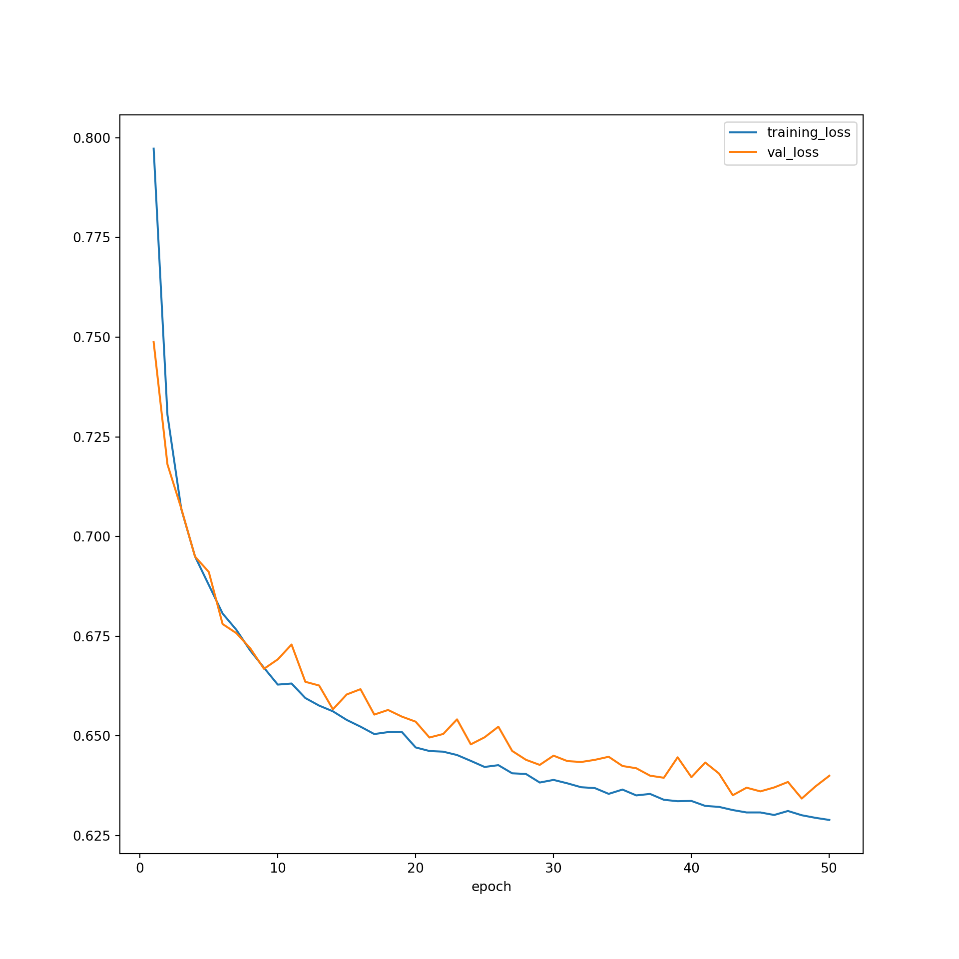
plt.rcParams['figure.figsize'] = [10, 10]
firstPlot = resultsDF.plot(x="epoch", y="training_f1")
resultsDF.plot(x='epoch', y="val_f1", ax=firstPlot)
plt.show()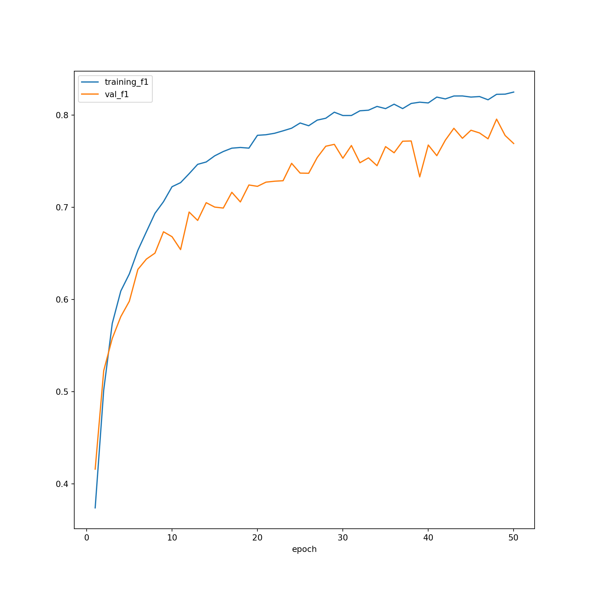
I will now validate the model using the withheld testing data. I first re-instantiate the model then load the model weights that were saved to disk. Again, these weights have been provided if you want to run the model validation code without training a model.
I instantiate a DataSet for the testing data without using the training augmentations then instantiate a DataLoader. I use torchmetrics to define a set of assessment metrics: overall accuracy, recall, precision, Kappa, and the confusion matrix. For the F1-score, recall, and precision metrics, I obtain the metric for each class as opposed to aggregating them to a single value by setting the average parameter to “none”.
To predict to the new data and calculate the metrics, I then loop over the testing mini-batches with the model in evaluation mode. Finally, I print the results.
The overall accuracy was pretty high (~90%). However, the class level F1-score, recall, and precision suggest that some classes were more difficult to predict. For example, the F1-score was lowest for the building (1) and road (4) classes. This could be because these classes were not as abundance in the dataset. Investigating the confusion matrix, you can see that there was some confusion between the background (0) and woodland (2) classes and also the roads (4) and background (0) classes.
model = myUNet(encoderChn=[16,32,64,128], decoderChn=[128,64,32,16], inChn=3, botChn=512, nCls=5).to(device)best_weights = torch.load('data/models/landcoverai_unet_model.pt')
model.load_state_dict(best_weights)<All keys matched successfully>testDS = MultiClassSegDataset(testDF, transform=test_transform)testDL = DataLoader(testDS, batch_size=8, shuffle=False, sampler=None,
batch_sampler=None, num_workers=0, collate_fn=None,
pin_memory=False, drop_last=True, timeout=0,
worker_init_fn=None)acc = tm.Accuracy(task="multiclass", num_classes=5, average="micro").to(device)
f1 = tm.F1Score(task="multiclass", num_classes=5, average='none').to(device)
recall = tm.Recall(task="multiclass", num_classes=5, average='none').to(device)
precision = tm.Precision(task="multiclass", num_classes=5, average='none').to(device)
kappa = tm.CohenKappa(task="multiclass", num_classes=5).to(device)
cm = tm.ConfusionMatrix(task="multiclass", num_classes=5).to(device)model.eval()myUNet(
(encoder1): Sequential(
(0): Conv2d(3, 16, kernel_size=(3, 3), stride=(1, 1), padding=(1, 1))
(1): BatchNorm2d(16, eps=1e-05, momentum=0.1, affine=True, track_running_stats=True)
(2): ReLU(inplace=True)
(3): Conv2d(16, 16, kernel_size=(3, 3), stride=(1, 1), padding=(1, 1))
(4): BatchNorm2d(16, eps=1e-05, momentum=0.1, affine=True, track_running_stats=True)
(5): ReLU(inplace=True)
)
(encoder2): Sequential(
(0): MaxPool2d(kernel_size=2, stride=2, padding=0, dilation=1, ceil_mode=False)
(1): Sequential(
(0): Conv2d(16, 32, kernel_size=(3, 3), stride=(1, 1), padding=(1, 1))
(1): BatchNorm2d(32, eps=1e-05, momentum=0.1, affine=True, track_running_stats=True)
(2): ReLU(inplace=True)
(3): Conv2d(32, 32, kernel_size=(3, 3), stride=(1, 1), padding=(1, 1))
(4): BatchNorm2d(32, eps=1e-05, momentum=0.1, affine=True, track_running_stats=True)
(5): ReLU(inplace=True)
)
)
(encoder3): Sequential(
(0): MaxPool2d(kernel_size=2, stride=2, padding=0, dilation=1, ceil_mode=False)
(1): Sequential(
(0): Conv2d(32, 64, kernel_size=(3, 3), stride=(1, 1), padding=(1, 1))
(1): BatchNorm2d(64, eps=1e-05, momentum=0.1, affine=True, track_running_stats=True)
(2): ReLU(inplace=True)
(3): Conv2d(64, 64, kernel_size=(3, 3), stride=(1, 1), padding=(1, 1))
(4): BatchNorm2d(64, eps=1e-05, momentum=0.1, affine=True, track_running_stats=True)
(5): ReLU(inplace=True)
)
)
(encoder4): Sequential(
(0): MaxPool2d(kernel_size=2, stride=2, padding=0, dilation=1, ceil_mode=False)
(1): Sequential(
(0): Conv2d(64, 128, kernel_size=(3, 3), stride=(1, 1), padding=(1, 1))
(1): BatchNorm2d(128, eps=1e-05, momentum=0.1, affine=True, track_running_stats=True)
(2): ReLU(inplace=True)
(3): Conv2d(128, 128, kernel_size=(3, 3), stride=(1, 1), padding=(1, 1))
(4): BatchNorm2d(128, eps=1e-05, momentum=0.1, affine=True, track_running_stats=True)
(5): ReLU(inplace=True)
)
)
(bottleneck): Sequential(
(0): MaxPool2d(kernel_size=2, stride=2, padding=0, dilation=1, ceil_mode=False)
(1): Sequential(
(0): Conv2d(128, 512, kernel_size=(3, 3), stride=(1, 1), padding=(1, 1))
(1): BatchNorm2d(512, eps=1e-05, momentum=0.1, affine=True, track_running_stats=True)
(2): ReLU(inplace=True)
(3): Conv2d(512, 512, kernel_size=(3, 3), stride=(1, 1), padding=(1, 1))
(4): BatchNorm2d(512, eps=1e-05, momentum=0.1, affine=True, track_running_stats=True)
(5): ReLU(inplace=True)
)
)
(decoder1up): Sequential(
(0): ConvTranspose2d(512, 512, kernel_size=(2, 2), stride=(2, 2))
(1): BatchNorm2d(512, eps=1e-05, momentum=0.1, affine=True, track_running_stats=True)
(2): ReLU(inplace=True)
)
(decoder1): Sequential(
(0): Conv2d(640, 128, kernel_size=(3, 3), stride=(1, 1), padding=(1, 1))
(1): BatchNorm2d(128, eps=1e-05, momentum=0.1, affine=True, track_running_stats=True)
(2): ReLU(inplace=True)
(3): Conv2d(128, 128, kernel_size=(3, 3), stride=(1, 1), padding=(1, 1))
(4): BatchNorm2d(128, eps=1e-05, momentum=0.1, affine=True, track_running_stats=True)
(5): ReLU(inplace=True)
)
(decoder2up): Sequential(
(0): ConvTranspose2d(128, 128, kernel_size=(2, 2), stride=(2, 2))
(1): BatchNorm2d(128, eps=1e-05, momentum=0.1, affine=True, track_running_stats=True)
(2): ReLU(inplace=True)
)
(decoder2): Sequential(
(0): Conv2d(192, 64, kernel_size=(3, 3), stride=(1, 1), padding=(1, 1))
(1): BatchNorm2d(64, eps=1e-05, momentum=0.1, affine=True, track_running_stats=True)
(2): ReLU(inplace=True)
(3): Conv2d(64, 64, kernel_size=(3, 3), stride=(1, 1), padding=(1, 1))
(4): BatchNorm2d(64, eps=1e-05, momentum=0.1, affine=True, track_running_stats=True)
(5): ReLU(inplace=True)
)
(decoder3up): Sequential(
(0): ConvTranspose2d(64, 64, kernel_size=(2, 2), stride=(2, 2))
(1): BatchNorm2d(64, eps=1e-05, momentum=0.1, affine=True, track_running_stats=True)
(2): ReLU(inplace=True)
)
(decoder3): Sequential(
(0): Conv2d(96, 32, kernel_size=(3, 3), stride=(1, 1), padding=(1, 1))
(1): BatchNorm2d(32, eps=1e-05, momentum=0.1, affine=True, track_running_stats=True)
(2): ReLU(inplace=True)
(3): Conv2d(32, 32, kernel_size=(3, 3), stride=(1, 1), padding=(1, 1))
(4): BatchNorm2d(32, eps=1e-05, momentum=0.1, affine=True, track_running_stats=True)
(5): ReLU(inplace=True)
)
(decoder4up): Sequential(
(0): ConvTranspose2d(32, 32, kernel_size=(2, 2), stride=(2, 2))
(1): BatchNorm2d(32, eps=1e-05, momentum=0.1, affine=True, track_running_stats=True)
(2): ReLU(inplace=True)
)
(decoder4): Sequential(
(0): Conv2d(48, 16, kernel_size=(3, 3), stride=(1, 1), padding=(1, 1))
(1): BatchNorm2d(16, eps=1e-05, momentum=0.1, affine=True, track_running_stats=True)
(2): ReLU(inplace=True)
(3): Conv2d(16, 16, kernel_size=(3, 3), stride=(1, 1), padding=(1, 1))
(4): BatchNorm2d(16, eps=1e-05, momentum=0.1, affine=True, track_running_stats=True)
(5): ReLU(inplace=True)
)
(classifier): Conv2d(16, 5, kernel_size=(1, 1), stride=(1, 1))
)with torch.no_grad():
for batch_idx, (inputs, targets) in enumerate(testDL):
inputs, targets = inputs.to(device), targets.to(device)
outputs = model(inputs)
#loss_v = criterion(outputs, targets)
accV = acc(outputs, targets)
f1V = f1(outputs, targets)
rV = recall(outputs, targets)
pV = precision(outputs, targets)
kappaV = kappa(outputs, targets)
cmV = cm(outputs, targets)
accV = acc.compute()
f1V = f1.compute()
rV = recall.compute()
pV = precision.compute()
kappaV = kappa.compute()
cmV = cm.compute()
acc.reset()
f1.reset()
recall.reset()
precision.reset()
kappa.reset()
cm.reset()print(accV)tensor(0.9222, device='cuda:0')print(f1V)tensor([0.9361, 0.8008, 0.9177, 0.9052, 0.6766], device='cuda:0')print(rV)tensor([0.9414, 0.7973, 0.9123, 0.8920, 0.6642], device='cuda:0')print(pV)tensor([0.9309, 0.8043, 0.9232, 0.9187, 0.6895], device='cuda:0')print(kappaV)tensor(0.8585, device='cuda:0')print(cmV)tensor([[225750755, 655920, 9904976, 1631765, 1856925],
[ 730452, 3154704, 24691, 16395, 30312],
[ 11989769, 11306, 131174200, 261049, 341827],
[ 2121916, 8914, 487192, 21753504, 16596],
[ 1915974, 91664, 498550, 14698, 4986346]],
device='cuda:0')Concluding Remarks
You have now seen how to train a semantic segmentation model to classify each individual pixel in an image. Fortunately, the training and validation process is not that different from those implemented for fully connected neural networks and convolutional neural networks for scene labeling, which were discussed in the prior modules.
In the next section, we will explore how to define UNets that use either VGGNet-16 or a ResNet architecture in the encoder.