Segmentation Model Package

Segmentation Models Package

Introduction

I feel that it is valuable to be able to define model architectures from scratch by subclassing nn.Module. However, there are many architectures available for different use cases and problem types. Also, you may want to have additional flexibility, such as the ability to change backbones or initialize using parameters obtained using pre-training. Also, some modern architectures can be very complicated and difficult to build from scratch. So, it would be desirable to have access to libraries that provide a wide variety of architectures and that offer flexibility. For semantic segmentation tasks, the Segmentation Models package provides these functionalities. This package is available at https://github.com/qubvel/segmentation_models.pytorch. We will explore the PyTorch implementation of this package specifically; however, there is also a Keras/Tensorflow version available: https://github.com/qubvel/segmentation_models.

Segmentation Models provides access to a wide variety of semantic segmentation architectures including UNet, UNet++, MANet, LinkNet, FPN, PSPNet, PAN, DeepLabv3, and DeepLabv3+. In this module, the demonstration will use DeepLabv3+. This package also provides a large number of CNN architectures that can be used as the encoder or backbone component of the semantic segmentation architecture including ResNet, ResNeXt, DenseNet, Inception, MobileNet, VGG, and Mix Vision Transformer. Pre-trained weights generated from different datasets are available. The number of different pre-trained weight sets available vary between the available CNN backbone architectures.

The user also has the ability to customize the architecture, and the settings available vary. For the DeepLabv3+ model, the user can specify which encoder to use, the number of stages or blocks in the encoder, if and which pre-trained weights to use, atrous rates, number of input channels, and number of classes being differentiated. There are also auxiliary parameters associated with the classification head auxiliary output component of the model. Interestingly, you can use pre-trained weights even if the number of current input channels is different from the data used to develop the pre-trained weights.

Outside of models, encoders, and pre-trained weights, this package also provides access to additional loss and assessment metrics applicable to semantic segmentation. It also provides methods to simplify the training loop.

Preparation

In this example, we will explore the binary classification problem of extracting surface mine extents from topographic maps. We will use the training, validation, and testing data developed in the prior module.

I import the standard data science packages: numpy, pandas, and matplotlib. I also import os for working with file paths, math, and OpenCV (cv2) for reading in the image data. For the deep learning-specific tasks, I read in torch, albumentations, torchmetrics, and Segmentation Models. Rasterio will be used to read the geospatial raster data for inference at the end of the training process. I also set the device to my available GPU. As in the prior CNN-based modules, the training process presented here is too computationally intensive for CPU-based computation.

import numpy as np
import pandas as pd
from matplotlib import pyplot as plt 
import os
import math
import cv2

import torch
import torch.nn as nn
from torch.utils.data.dataset import Dataset
from torch.utils.data import DataLoader

import albumentations as A

import segmentation_models_pytorch as smp

import torchmetrics as tm

import rasterio as rio
from rasterio.plot import show

device = torch.device("cuda:0" if torch.cuda.is_available() else "cpu")
print(device)

cuda:0

I next read in the CSV files that were created in the prior module and contain information for each chip in the training, testing, and validation datasets as pandas dataframes. Printing the lengths of these dataframes provides the number of available chips or samples in each partition. Checking the column names, the path to the image chip is housed in the 3rd column while the path to the mask is housed in the 4th column. The “division” column notes whether the chip was a background-only sample or if it contained some pixels mapped to the positive class.

folder = "C:/myFiles/work/topo_dl_data/topo_dl_data/processing/"
train = pd.read_csv(folder + "trainDF.csv")
val = pd.read_csv(folder + "valDF.csv")
test = pd.read_csv(folder + "testDF.csv")

len(train)

49842

len(val)

11826

len(test)

10692

train.columns

Index(['Unnamed: 0', 'chpN', 'chpPath', 'mskPth', 'division'], dtype='object')

On issue with the training set is that there is a large number of background-only chips. To deal with class imbalance, I will only use a subsample of the available background-only chips. This is accomplished by separating the background-only and presence samples into separate dataframes, sampling 2,000 background chips from the larger set without replacement, and merging the presence and subset of background-only chips into a new dataframe. This subset will be used to train the model.

train.groupby(['division'])['division'].count()

division
Background    42071
Positive       7771
Name: division, dtype: int64

trainP = train.query('division == "Positive"')
trainB = train.query("division == 'Background'")
trainB = trainB.sample(n=2000, replace=False)
train2 = pd.concat([trainP, trainB])

train2.groupby(['division'])['division'].count()

division
Background    2000
Positive      7771
Name: division, dtype: int64

I next define a DataSet subclass to read in and convert the image chips and associated masks to tensors. Here are a few notes about the DataSet subclass.

1. The path to the image chip is read from the third column (index 2).
2. The path to the mask is read from the fourth column (index 3).
3. Since cv2 reads images using a channels-last configuration, I must use permute() to convert the tensors to channels-first.
4. The model will expect the image mini-batches to have a shape of (Mini-Batch, Channels, Height, Width), a 32-bit float data type, and be scaled from 0 to 1. To rescale the 8-bit data, the values are divided by 255.
5. The model will expect the mask mini-batches to have a shape of (Mini-Batch, Height, Width), a long integer data type, and have unique codes for each class. In this case, the original data assigns 255 to the surface disturbance class and 0 to the background. Dividing by 255 rescales the data from 0 to 1 where 1 indicates the positive case and 0 indicates the background.

# Subclass and define custom dataset ===========================
class SegData(Dataset):
    
    def __init__(self, df, transform=None):
        self.df = df
        self.transform = transform
        
    def __getitem__(self, idx):
        image_name = self.df.iloc[idx, 2]
        mask_name = self.df.iloc[idx, 3]
        image = cv2.imread(image_name)
        image = cv2.cvtColor(image, cv2.COLOR_BGR2RGB)
        mask = cv2.imread(mask_name, cv2.IMREAD_UNCHANGED)
        image = image.astype('uint8')
        mask = mask.astype('uint8')
        mask = np.expand_dims(mask, axis=2)
        
        if(self.transform is not None):
            transformed = self.transform(image=image, mask=mask)
            image = transformed["image"]
            mask = transformed["mask"]
            image = torch.from_numpy(image)
            mask = torch.from_numpy(mask)   
            image = image.permute(2, 0, 1)
            image = image.float()/255
            mask = mask.permute(2, 0, 1)
            mask = mask.float()/255
            mask = mask.squeeze().long()
        else: 
            image = torch.from_numpy(image)
            mask = torch.from_numpy(mask)
            image = image.permute(2, 0, 1)
            image = image.float()/255
            mask = mask.permute(2, 0, 1)
            mask = mask.float()/255
            mask = mask.squeeze().long()
        return image, mask  
    def __len__(self):  
        return len(self.df)

The albumentations package is used to define data augmentations to potentially reduce overfitting. Specifically, random changes to brightness and contrast are applied along with random horizontal and vertical flips and median blurring.

train_transform = A.Compose(
    [
        A.RandomBrightnessContrast(brightness_limit=0.3, contrast_limit=0.3, p=0.5),
        A.HorizontalFlip(p=0.5),
        A.VerticalFlip(p=0.5),
        A.MedianBlur(blur_limit=3, always_apply=False, p=0.1),
    ]
)

I next instantiate the training and validation DataSet instances with the data augmentations applied to only the training data. The DataLoaders are defined using a mini-batch size of 16, which worked on my architecture. You may need to change this based on your resources.

trainDS = SegData(train2, transform=train_transform)
valDS = SegData(val, transform=None)
print("Number of Training Samples: " + str(len(trainDS)) + " Number of Validation Samples: " + str(len(valDS)))

Number of Training Samples: 9771 Number of Validation Samples: 11826

trainDL = torch.utils.data.DataLoader(trainDS, batch_size=16, shuffle=True, num_workers=0, drop_last=True)
valDL =  torch.utils.data.DataLoader(valDS, batch_size=16, shuffle=False, num_workers=0, drop_last=True)

I plot information about the mini-batches and an individual image and associated mask as checks. The generated mini-batches and individual images have the correct shapes and data types.

I then plot an image and associated mask. I must permute the bands since matplotlib expects the data to be in a channels-last as opposed to channels-first configuration. It looks like these data are being read and converted to tensors correctly.

batch = next(iter(trainDL))
images, labels = batch
print(images.shape, labels.shape, type(images), type(labels), images.dtype, labels.dtype)

torch.Size([16, 3, 256, 256]) torch.Size([16, 256, 256]) <class 'torch.Tensor'> <class 'torch.Tensor'> torch.float32 torch.int64

testImg = images[1]
testMsk = labels[1]
print(testImg.shape, testImg.dtype, type(testImg), testMsk.shape, 
testMsk.dtype, type(testMsk), testImg.min(), 
testImg.max(), testMsk.min(), testMsk.max())

torch.Size([3, 256, 256]) torch.float32 <class 'torch.Tensor'> torch.Size([256, 256]) torch.int64 <class 'torch.Tensor'> tensor(0.) tensor(1.) tensor(0) tensor(1)

trainDSP = SegData(trainP, transform=None)
trainDLP = torch.utils.data.DataLoader(trainDSP, batch_size=16, shuffle=True, num_workers=0, drop_last=True)
batch = next(iter(trainDLP))
images, labels = batch
testImg = images[1]
testMsk = labels[1]

# Plot example image =====================================
plt.imshow(testImg.permute(1,2,0))
plt.show()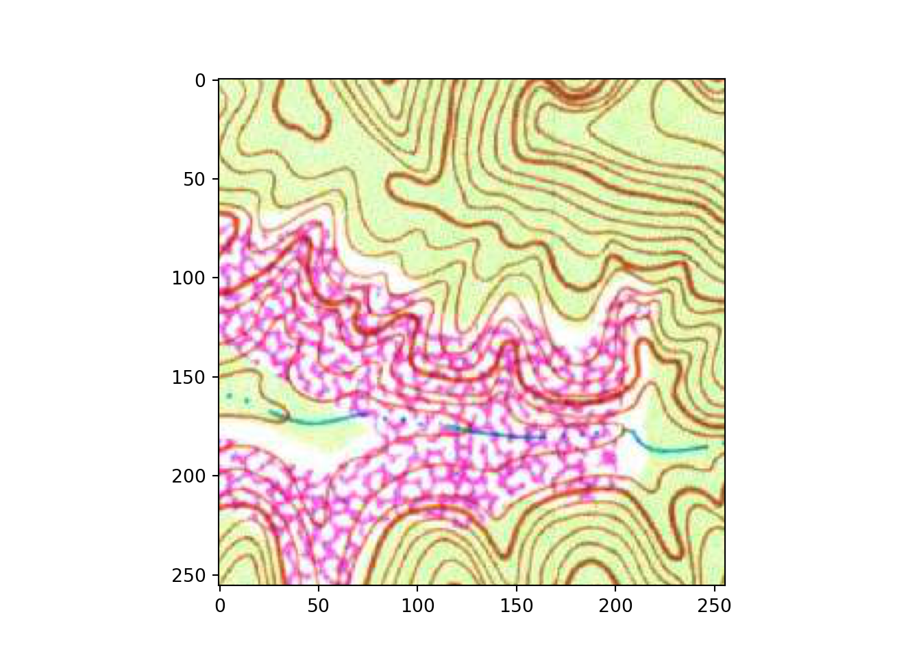

# Plot example image =====================================
plt.imshow(testMsk.unsqueeze(dim=0).permute(1,2,0))
plt.show()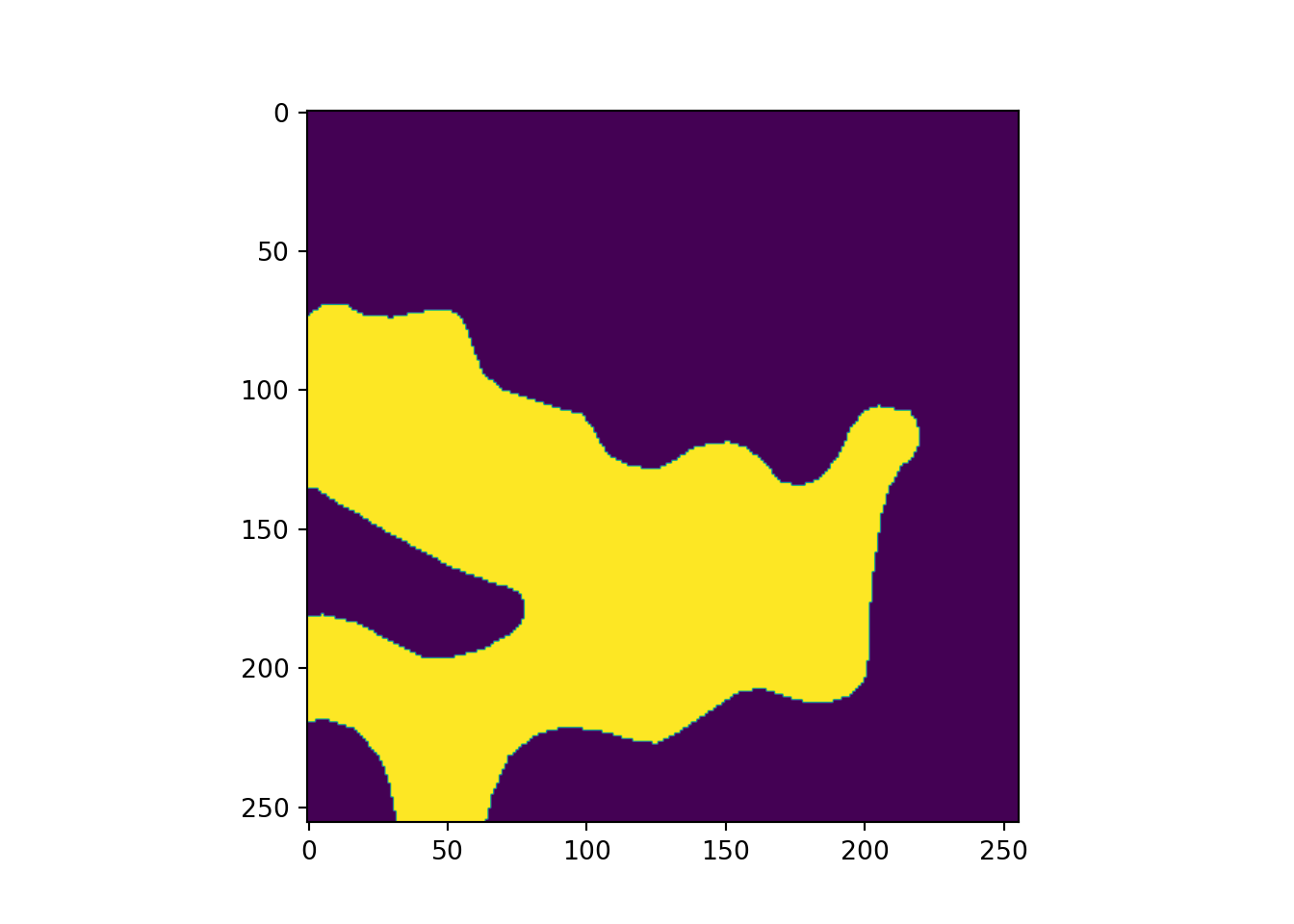

DeepLabv3+

The DeepLabv3+ semantic segmentation architecture is initiated using the DeepLabV3Plus() function from Segmentation Models. Since the Segmentation Models package includes this architecture, this function can be called to instantiate an instance of DeepLabv3+ as opposed to building it on your own by subclassing nn.Module. I specify the name of the encoder (“ResNet-32”), and I do not instantiate using pre-trained weights since this is a very different problem than the ImageNet classification problem. No activation function (i.e., softmax) is used so that raw logits are delivered.

Since this is a binary classification problem, I could define the model to return only a logit for the positive class or logits for both the positive and background classes. In this example, I have chosen to treat the problem the same as a multiclass classification problem, so logits will be returned for both the positive and background class.

encoder = "resnet18"
encoder_weights = None
activation = None

model = smp.DeepLabV3Plus(
    encoder_name=encoder, 
    encoder_weights=encoder_weights, 
    classes=2, 
    activation=activation,
).to(device)

Train Model

The Segmentation Models package provides some tools to simplify the training loop. However, here I will make use of our standard training loop, which has been discussed and implemented multiple times in prior modules. You can consult the package documentation if you are interested in learning more about the provided TrainEpoch() and ValidEpoch() classes provided by Segmentation Models.

I first initialize an instance of the cross entropy loss as implemented in PyTorch. I will use the AdamW optimizer with the default learning rate. I will monitor the overall accuracy, class-aggregated, macro-averaged F1-score, and Kappa statistic as implemented with torchmetrics. The model will run for a total of 50 epochs, and the saved model will only be overwritten if the class-aggregated F1-score improves for the validation data.

In this example, all parameters are trainable since none have been frozen. If you initialize the model using pre-trained weights, the default behavior is that all parameters will also be updateable. If you want to freeze or unfreeze the backbone or encoder weights, you can use the functions provided below and obtained at the commented-out URL.

If you choose to run the training loop, it will take some time. It took roughly 5 hours to run on my machine with a single GPU. We have provided a trained model if you want to run the later code without training the model.

criterion = nn.CrossEntropyLoss()

optimizer = torch.optim.AdamW(model.parameters())

acc = tm.Accuracy(task="multiclass", average="micro", num_classes=2).to(device)
f1 = tm.F1Score(task="multiclass", average="macro", num_classes=2).to(device)
kappa = tm.CohenKappa(task="multiclass", average = "micro", num_classes=2).to(device)

epochs = 50
saveFolder = "C:/myFiles/work/dl/topoDL_models_2/"

#https://github.com/qubvel/segmentation_models.pytorch/issues/79 
def freeze_encoder(model):
    for child in model.encoder.children():
        for param in child.parameters():
            param.requires_grad = False
    return

def unfreeze(model):
    for child in model.children():
        for param in child.parameters():
            param.requires_grad = True
    return

eNum = []
t_loss = []
t_acc = []
t_f1 = []
t_kappa = []
v_loss = []
v_acc = []
v_f1 = []
v_kappa = []

f1VMax = 0.0

model.train()
#Initiate running loss for epoch
running_loss = 0.0
# Loop over epochs
for epoch in range(1, epochs+1):
    # Loop over training batches
    for batch_idx, (inputs, targets) in enumerate(trainDL):
        # Get data and move to device
        inputs, targets = inputs.to(device), targets.to(device)

        # Clear gradients
        optimizer.zero_grad()
        # Predict data
        outputs = model(inputs)
        # Calculate loss
        loss = criterion(outputs, targets)

        # Calculate metrics
        accT = acc(outputs, targets)
        f1T = f1(outputs, targets)
        kappaT = kappa(outputs, targets)
        
        # Backpropagate
        loss.backward()

        # Update parameters
        optimizer.step()

        #Update running with batch results
        running_loss += loss.item()

    # Accumulate loss and metrics at end of training epoch
    epoch_loss = running_loss/len(trainDL)
    accT = acc.compute()
    f1T = f1.compute()
    kappaT = kappa.compute()

    # Print Losses and metrics at end of each training epoch   
    print(f'Epoch: {epoch}, Training Loss: {epoch_loss:.4f}, Training Accuracy: {accT:.4f}, Training F1: {f1T:.4f}, Training Kappa: {kappaT:.4f}')

    # Append results
    eNum.append(epoch)
    t_loss.append(epoch_loss)
    t_acc.append(accT.detach().cpu().numpy())
    t_f1.append(f1T.detach().cpu().numpy())
    t_kappa.append(kappaT.detach().cpu().numpy())

    # Reset metrics
    acc.reset()
    f1.reset()
    kappa.reset()

    # loop over validation batches
    with torch.no_grad():
        #Initialize running validation loss
        running_loss_v = 0.0
        for batch_idx, (inputs, targets) in enumerate(valDL):
            # Get data and move to device
            inputs, targets = inputs.to(device), targets.to(device)

            # Predict data
            outputs = model(inputs)
            # Calculate validation loss
            loss_v = criterion(outputs, targets)
            
            #Update running with batch results
            running_loss_v += loss_v.item()

            # Calculate metrics
            accV = acc(outputs, targets)
            f1V = f1(outputs, targets)
            kappaV = kappa(outputs, targets)
            
    #Accumulate loss and metrics at end of validation epoch
    epoch_loss_v = running_loss_v/len(valDL)
    accV = acc.compute()
    f1V = f1.compute()
    kappaV = kappa.compute()

    # Print validation loss and metrics
    print(f'Validation Loss: {epoch_loss_v:.4f}, Validation Accuracy: {accV:.4f}, Validation F1: {f1V:.4f}, Validation Kappa: {kappaV:.4f}')

    # Append results
    v_loss.append(epoch_loss_v)
    v_acc.append(accV.detach().cpu().numpy())
    v_f1.append(f1V.detach().cpu().numpy())
    v_kappa.append(kappaV.detach().cpu().numpy())

    # Reset metrics
    acc.reset()
    f1.reset()
    kappa.reset()

    # Save model if validation F1-score improves
    f1V2 = f1V.detach().cpu().numpy()
    if f1V2 > f1VMax:
        f1VMax = f1V2
        torch.save(model.state_dict(), saveFolder + 'topoDL_dlv3p_model.pt')
        print(f'Model saved for epoch {epoch}.')

SeNum = pd.Series(eNum, name="epoch")
St_loss = pd.Series(t_loss, name="training_loss")
St_acc = pd.Series(t_acc, name="training_accuracy")
St_f1 = pd.Series(t_f1, name="training_f1")
St_kappa = pd.Series(t_kappa, name="training_kappa")
Sv_loss = pd.Series(v_loss, name="val_loss")
Sv_acc = pd.Series(v_acc, name="val_accuracy")
Sv_f1 = pd.Series(v_f1, name="val_f1")
Sv_kappa = pd.Series(v_kappa, name="val_kappa")
resultsDF = pd.concat([SeNum, St_loss, St_acc, St_f1, St_kappa, Sv_loss, Sv_acc, Sv_f1, Sv_kappa], axis=1)

resultsDF.to_csv(saveFolder+"resultsTopoDL.csv")

resultsDF = pd.read_csv("data/models/resultsTopoDL.csv")

Once the model training is completed, I explore the training process by plotting the training and validation losses over the training epochs and the training and validation F1-scores.

plt.rcParams['figure.figsize'] = [10, 10]
firstPlot = resultsDF.plot(x='epoch', y="training_loss")
resultsDF.plot(x='epoch', y="val_loss", ax=firstPlot)
plt.show()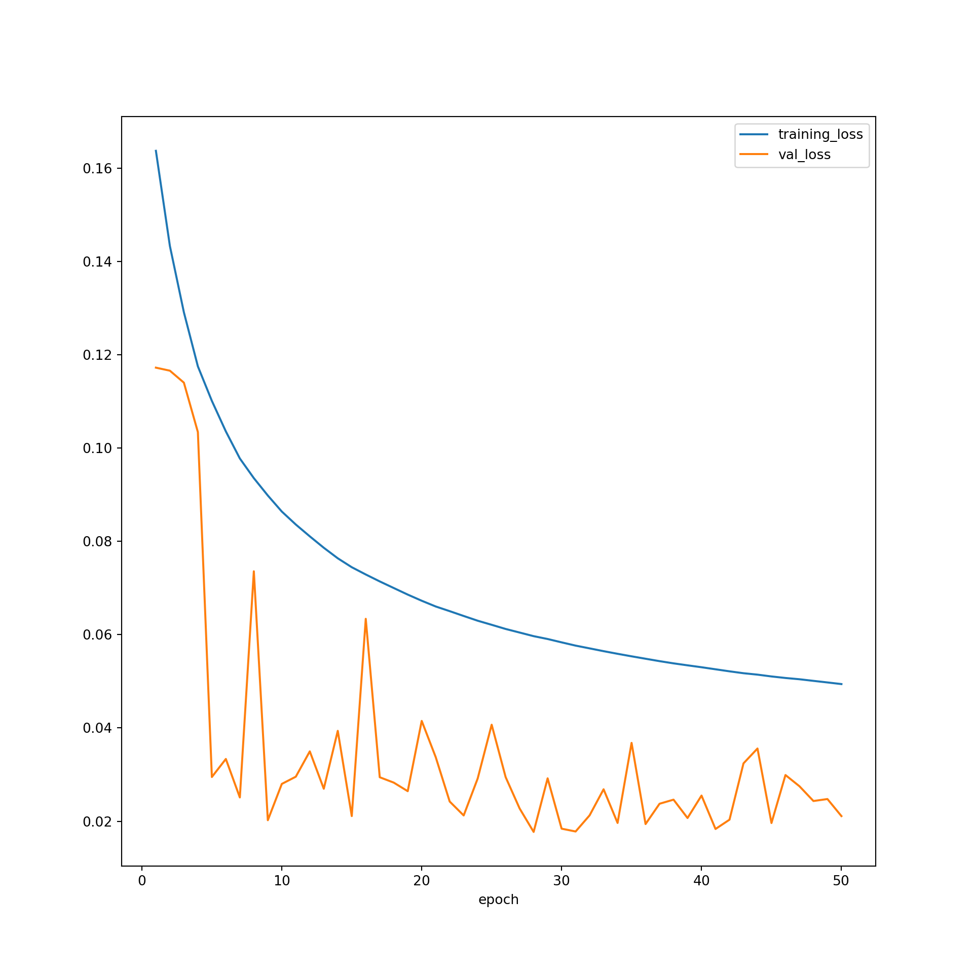

plt.rcParams['figure.figsize'] = [10, 10]
firstPlot = resultsDF.plot(x="epoch", y="training_f1")
resultsDF.plot(x='epoch', y="val_f1", ax=firstPlot)
plt.show()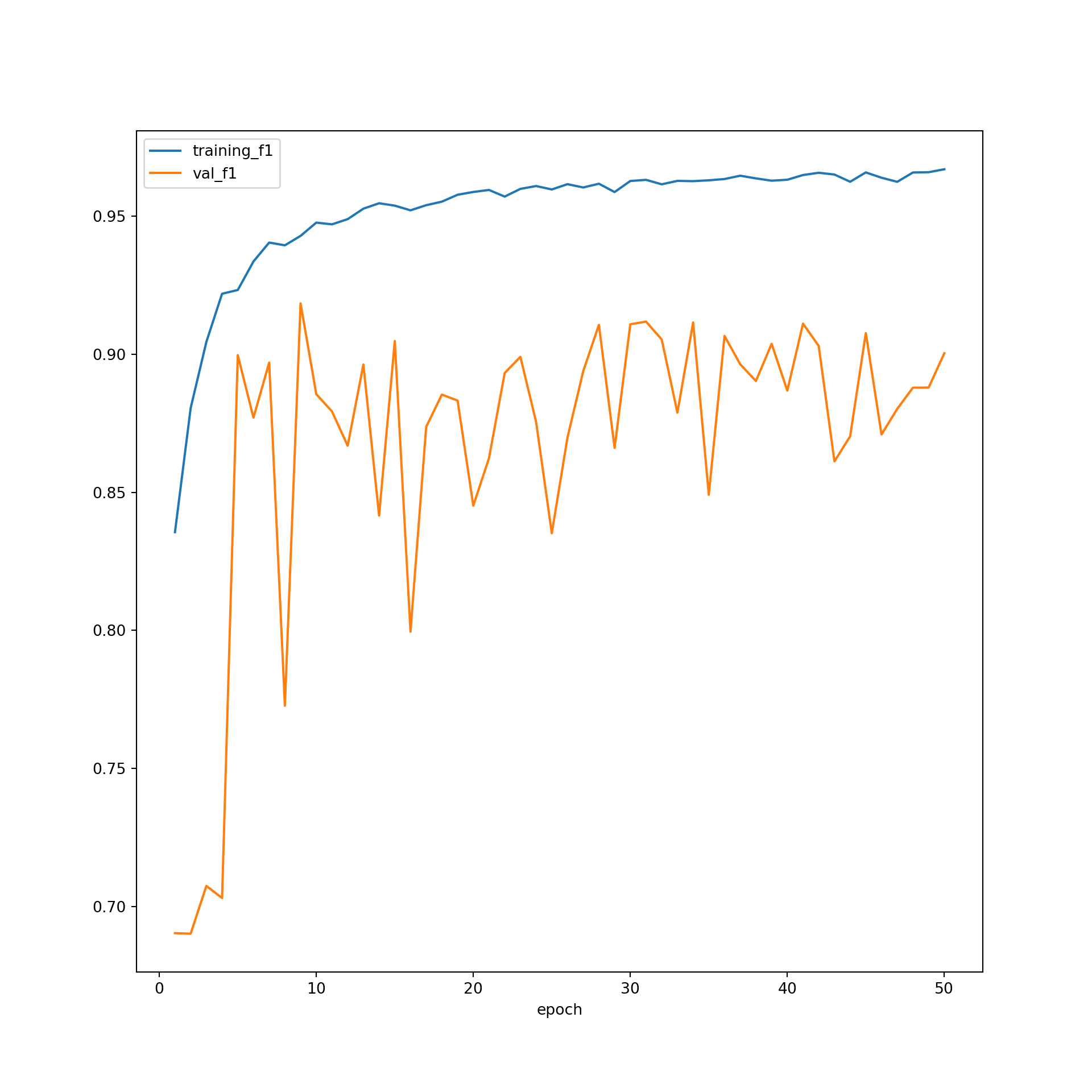

Assess Model

Once the model is trained, it can be used to perform inference on new data. I will demonstrate assessing the model using the withheld testing data. This involves the following steps:

1. Redefine the model and load in the learned parameters from disk
2. Instantiate a DataSet for the testing data
3. Define a DataLoader for the testing data
4. Initialize assessment metrics provided by torchmetrics
5. Execute a loop to predict the testing samples and calculate and accumulate the assessment metrics over multiple epochs

model = smp.DeepLabV3Plus(
    encoder_name=encoder, 
    encoder_weights=encoder_weights, 
    classes=2, 
    activation=activation,
).to(device)

model.load_state_dict(torch.load("data/models/topoDL_dlv3p_model.pt"))

<All keys matched successfully>

testDS = SegData(test, transform=None)

testDL =  torch.utils.data.DataLoader(testDS, batch_size=16, shuffle=False, num_workers=0, drop_last=True)

acc = tm.Accuracy(task="multiclass", num_classes=2).to(device)
f1 = tm.F1Score(task="multiclass", num_classes=2, average='none').to(device)
recall = tm.Recall(task="multiclass", num_classes=2, average='none').to(device)
precision = tm.Precision(task="multiclass", num_classes=2, average='none').to(device)
kappa = tm.CohenKappa(task="multiclass", num_classes=2).to(device)
cm = tm.ConfusionMatrix(task="multiclass", num_classes=2).to(device)

model.eval()

DeepLabV3Plus(
  (encoder): ResNetEncoder(
    (conv1): Conv2d(3, 64, kernel_size=(7, 7), stride=(2, 2), padding=(3, 3), bias=False)
    (bn1): BatchNorm2d(64, eps=1e-05, momentum=0.1, affine=True, track_running_stats=True)
    (relu): ReLU(inplace=True)
    (maxpool): MaxPool2d(kernel_size=3, stride=2, padding=1, dilation=1, ceil_mode=False)
    (layer1): Sequential(
      (0): BasicBlock(
        (conv1): Conv2d(64, 64, kernel_size=(3, 3), stride=(1, 1), padding=(1, 1), bias=False)
        (bn1): BatchNorm2d(64, eps=1e-05, momentum=0.1, affine=True, track_running_stats=True)
        (relu): ReLU(inplace=True)
        (conv2): Conv2d(64, 64, kernel_size=(3, 3), stride=(1, 1), padding=(1, 1), bias=False)
        (bn2): BatchNorm2d(64, eps=1e-05, momentum=0.1, affine=True, track_running_stats=True)
      )
      (1): BasicBlock(
        (conv1): Conv2d(64, 64, kernel_size=(3, 3), stride=(1, 1), padding=(1, 1), bias=False)
        (bn1): BatchNorm2d(64, eps=1e-05, momentum=0.1, affine=True, track_running_stats=True)
        (relu): ReLU(inplace=True)
        (conv2): Conv2d(64, 64, kernel_size=(3, 3), stride=(1, 1), padding=(1, 1), bias=False)
        (bn2): BatchNorm2d(64, eps=1e-05, momentum=0.1, affine=True, track_running_stats=True)
      )
    )
    (layer2): Sequential(
      (0): BasicBlock(
        (conv1): Conv2d(64, 128, kernel_size=(3, 3), stride=(2, 2), padding=(1, 1), bias=False)
        (bn1): BatchNorm2d(128, eps=1e-05, momentum=0.1, affine=True, track_running_stats=True)
        (relu): ReLU(inplace=True)
        (conv2): Conv2d(128, 128, kernel_size=(3, 3), stride=(1, 1), padding=(1, 1), bias=False)
        (bn2): BatchNorm2d(128, eps=1e-05, momentum=0.1, affine=True, track_running_stats=True)
        (downsample): Sequential(
          (0): Conv2d(64, 128, kernel_size=(1, 1), stride=(2, 2), bias=False)
          (1): BatchNorm2d(128, eps=1e-05, momentum=0.1, affine=True, track_running_stats=True)
        )
      )
      (1): BasicBlock(
        (conv1): Conv2d(128, 128, kernel_size=(3, 3), stride=(1, 1), padding=(1, 1), bias=False)
        (bn1): BatchNorm2d(128, eps=1e-05, momentum=0.1, affine=True, track_running_stats=True)
        (relu): ReLU(inplace=True)
        (conv2): Conv2d(128, 128, kernel_size=(3, 3), stride=(1, 1), padding=(1, 1), bias=False)
        (bn2): BatchNorm2d(128, eps=1e-05, momentum=0.1, affine=True, track_running_stats=True)
      )
    )
    (layer3): Sequential(
      (0): BasicBlock(
        (conv1): Conv2d(128, 256, kernel_size=(3, 3), stride=(2, 2), padding=(1, 1), bias=False)
        (bn1): BatchNorm2d(256, eps=1e-05, momentum=0.1, affine=True, track_running_stats=True)
        (relu): ReLU(inplace=True)
        (conv2): Conv2d(256, 256, kernel_size=(3, 3), stride=(1, 1), padding=(1, 1), bias=False)
        (bn2): BatchNorm2d(256, eps=1e-05, momentum=0.1, affine=True, track_running_stats=True)
        (downsample): Sequential(
          (0): Conv2d(128, 256, kernel_size=(1, 1), stride=(2, 2), bias=False)
          (1): BatchNorm2d(256, eps=1e-05, momentum=0.1, affine=True, track_running_stats=True)
        )
      )
      (1): BasicBlock(
        (conv1): Conv2d(256, 256, kernel_size=(3, 3), stride=(1, 1), padding=(1, 1), bias=False)
        (bn1): BatchNorm2d(256, eps=1e-05, momentum=0.1, affine=True, track_running_stats=True)
        (relu): ReLU(inplace=True)
        (conv2): Conv2d(256, 256, kernel_size=(3, 3), stride=(1, 1), padding=(1, 1), bias=False)
        (bn2): BatchNorm2d(256, eps=1e-05, momentum=0.1, affine=True, track_running_stats=True)
      )
    )
    (layer4): Sequential(
      (0): BasicBlock(
        (conv1): Conv2d(256, 512, kernel_size=(3, 3), stride=(1, 1), padding=(2, 2), dilation=(2, 2), bias=False)
        (bn1): BatchNorm2d(512, eps=1e-05, momentum=0.1, affine=True, track_running_stats=True)
        (relu): ReLU(inplace=True)
        (conv2): Conv2d(512, 512, kernel_size=(3, 3), stride=(1, 1), padding=(2, 2), dilation=(2, 2), bias=False)
        (bn2): BatchNorm2d(512, eps=1e-05, momentum=0.1, affine=True, track_running_stats=True)
        (downsample): Sequential(
          (0): Conv2d(256, 512, kernel_size=(1, 1), stride=(1, 1), dilation=(2, 2), bias=False)
          (1): BatchNorm2d(512, eps=1e-05, momentum=0.1, affine=True, track_running_stats=True)
        )
      )
      (1): BasicBlock(
        (conv1): Conv2d(512, 512, kernel_size=(3, 3), stride=(1, 1), padding=(2, 2), dilation=(2, 2), bias=False)
        (bn1): BatchNorm2d(512, eps=1e-05, momentum=0.1, affine=True, track_running_stats=True)
        (relu): ReLU(inplace=True)
        (conv2): Conv2d(512, 512, kernel_size=(3, 3), stride=(1, 1), padding=(2, 2), dilation=(2, 2), bias=False)
        (bn2): BatchNorm2d(512, eps=1e-05, momentum=0.1, affine=True, track_running_stats=True)
      )
    )
  )
  (decoder): DeepLabV3PlusDecoder(
    (aspp): Sequential(
      (0): ASPP(
        (convs): ModuleList(
          (0): Sequential(
            (0): Conv2d(512, 256, kernel_size=(1, 1), stride=(1, 1), bias=False)
            (1): BatchNorm2d(256, eps=1e-05, momentum=0.1, affine=True, track_running_stats=True)
            (2): ReLU()
          )
          (1): ASPPSeparableConv(
            (0): SeparableConv2d(
              (0): Conv2d(512, 512, kernel_size=(3, 3), stride=(1, 1), padding=(12, 12), dilation=(12, 12), groups=512, bias=False)
              (1): Conv2d(512, 256, kernel_size=(1, 1), stride=(1, 1), bias=False)
            )
            (1): BatchNorm2d(256, eps=1e-05, momentum=0.1, affine=True, track_running_stats=True)
            (2): ReLU()
          )
          (2): ASPPSeparableConv(
            (0): SeparableConv2d(
              (0): Conv2d(512, 512, kernel_size=(3, 3), stride=(1, 1), padding=(24, 24), dilation=(24, 24), groups=512, bias=False)
              (1): Conv2d(512, 256, kernel_size=(1, 1), stride=(1, 1), bias=False)
            )
            (1): BatchNorm2d(256, eps=1e-05, momentum=0.1, affine=True, track_running_stats=True)
            (2): ReLU()
          )
          (3): ASPPSeparableConv(
            (0): SeparableConv2d(
              (0): Conv2d(512, 512, kernel_size=(3, 3), stride=(1, 1), padding=(36, 36), dilation=(36, 36), groups=512, bias=False)
              (1): Conv2d(512, 256, kernel_size=(1, 1), stride=(1, 1), bias=False)
            )
            (1): BatchNorm2d(256, eps=1e-05, momentum=0.1, affine=True, track_running_stats=True)
            (2): ReLU()
          )
          (4): ASPPPooling(
            (0): AdaptiveAvgPool2d(output_size=1)
            (1): Conv2d(512, 256, kernel_size=(1, 1), stride=(1, 1), bias=False)
            (2): BatchNorm2d(256, eps=1e-05, momentum=0.1, affine=True, track_running_stats=True)
            (3): ReLU()
          )
        )
        (project): Sequential(
          (0): Conv2d(1280, 256, kernel_size=(1, 1), stride=(1, 1), bias=False)
          (1): BatchNorm2d(256, eps=1e-05, momentum=0.1, affine=True, track_running_stats=True)
          (2): ReLU()
          (3): Dropout(p=0.5, inplace=False)
        )
      )
      (1): SeparableConv2d(
        (0): Conv2d(256, 256, kernel_size=(3, 3), stride=(1, 1), padding=(1, 1), groups=256, bias=False)
        (1): Conv2d(256, 256, kernel_size=(1, 1), stride=(1, 1), bias=False)
      )
      (2): BatchNorm2d(256, eps=1e-05, momentum=0.1, affine=True, track_running_stats=True)
      (3): ReLU()
    )
    (up): UpsamplingBilinear2d(scale_factor=4.0, mode=bilinear)
    (block1): Sequential(
      (0): Conv2d(64, 48, kernel_size=(1, 1), stride=(1, 1), bias=False)
      (1): BatchNorm2d(48, eps=1e-05, momentum=0.1, affine=True, track_running_stats=True)
      (2): ReLU()
    )
    (block2): Sequential(
      (0): SeparableConv2d(
        (0): Conv2d(304, 304, kernel_size=(3, 3), stride=(1, 1), padding=(1, 1), groups=304, bias=False)
        (1): Conv2d(304, 256, kernel_size=(1, 1), stride=(1, 1), bias=False)
      )
      (1): BatchNorm2d(256, eps=1e-05, momentum=0.1, affine=True, track_running_stats=True)
      (2): ReLU()
    )
  )
  (segmentation_head): SegmentationHead(
    (0): Conv2d(256, 2, kernel_size=(1, 1), stride=(1, 1))
    (1): UpsamplingBilinear2d(scale_factor=4.0, mode=bilinear)
    (2): Activation(
      (activation): Identity()
    )
  )
)

with torch.no_grad():
    for batch_idx, (inputs, targets) in enumerate(testDL):
        inputs, targets = inputs.to(device), targets.to(device)
        outputs = model(inputs)
        #loss_v = criterion(outputs, targets)
        accV = acc(outputs, targets)
        f1V = f1(outputs, targets)
        rV = recall(outputs, targets)
        pV = precision(outputs, targets)
        kappaV = kappa(outputs, targets)
        cmV = cm(outputs, targets)
accV = acc.compute()
f1V = f1.compute()
rV = recall.compute()
pV = precision.compute()
kappaV = kappa.compute()
cmV = cm.compute()
acc.reset()
f1.reset()
recall.reset()
precision.reset()
kappa.reset()
cm.reset()

Generally, the assessment suggests strong model performance. This is expected since the pattern representing surface mining is very unique or differentiable from the background features.

print(accV)

tensor(0.9972, device='cuda:0')

print(f1V)

tensor([0.9986, 0.9129], device='cuda:0')

print(rV)

tensor([0.9985, 0.9168], device='cuda:0')

print(pV)

tensor([0.9986, 0.9089], device='cuda:0')

print(kappaV)

tensor(0.9114, device='cuda:0')

print(cmV)

tensor([[688103214,   1038740],
        [   940327,  10366487]], device='cuda:0')

Spatial Prediction

Once a model is trained, it can be used to infer back to entire image extents as opposed to individual image chips. We explored making spatial predictions using the landcover.ai dataset in a prior module. Here, I will demonstrate the same process for this classification problem. I first define a topographic map that I want to predict to that was included as part of the testing datasets. Plotting the topographic map, you can see that some surface disturbance extents are present.

testImg = "data/files/KY_Dorton_708542_1954_24000_geo.tif"

src = rio.open(testImg)
rio.plot.show(src)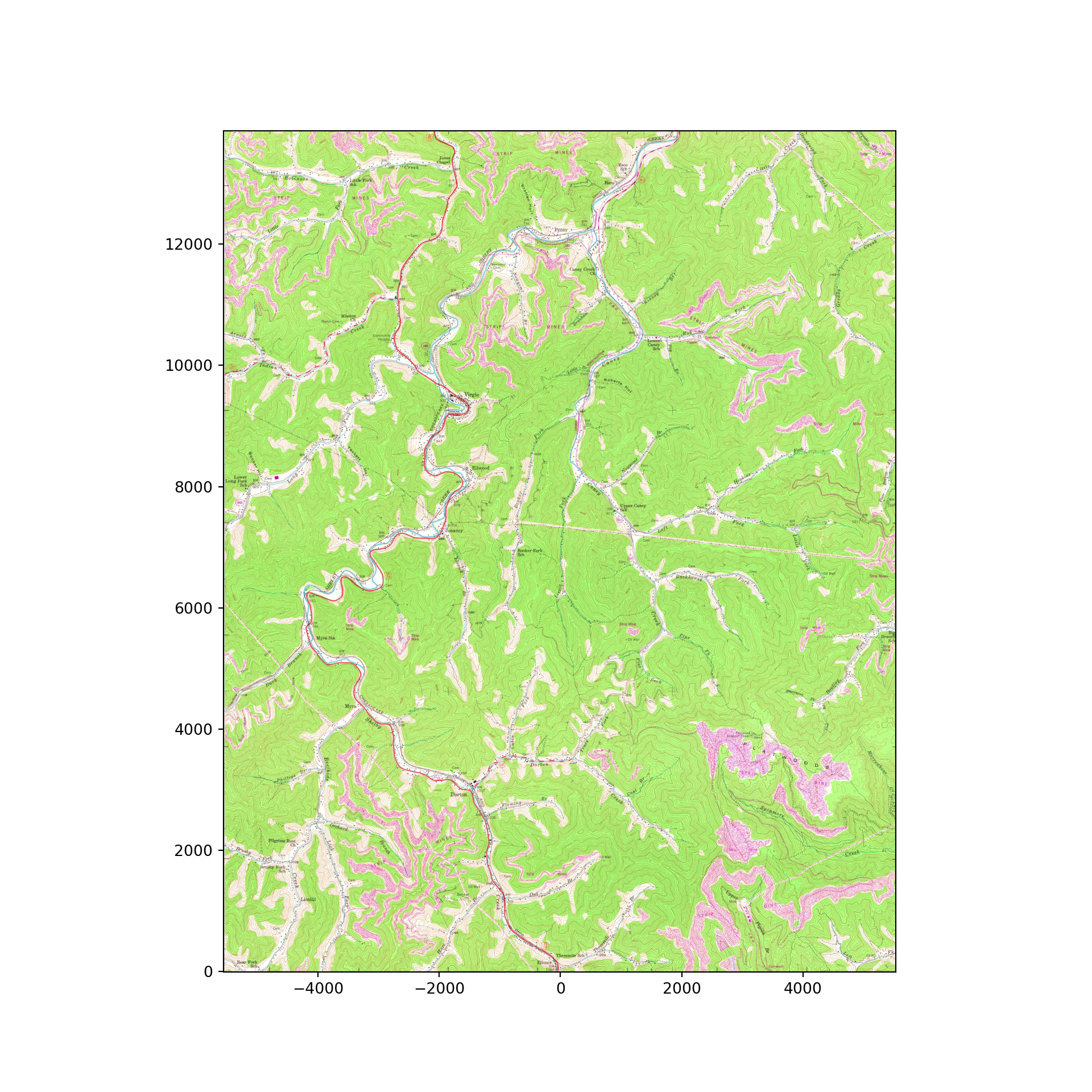

src.close()

I next redefine the geoInfer() function that was explored in the prior module that can make predictions on overlapping image chips, crop off outer rows and columns of pixels, and merge the predictions back to a single raster file that is georeferenced and has an associated coordinate reference system. I then use this function and the trained model to predict the example topographic map.

def geoInfer(image_in, pred_out, chip_size, stride_x, stride_y, crop, n_channels):

    #Read in topo map and convert to tensor===========================
    image1 = cv2.imread(image_in)
    image1 = cv2.cvtColor(image1, cv2.COLOR_BGR2RGB)
    image1 = image1.astype('uint8')
    image1 = torch.from_numpy(image1)
    image1 = image1.permute(2, 0, 1)
    image1 = image1.float()/255
    t_arr = image1
    
    #Make blank grid to write predictions two with same height and width as topo===========================
    image2 = cv2.imread(image_in)
    image2 = cv2.cvtColor(image2, cv2.COLOR_BGR2RGB)
    image2 = image2.astype('uint8')
    image2 = torch.from_numpy(image2)
    image2 = image2.permute(2, 0, 1)
    image2 = image2.float()/255
    p_arr = image2[0, :, :]
    p_arr[:,:] = 0
    
    #Predict to entire topo using overlapping chips, merge back to original extent=============
    size = chip_size
    stride_x = stride_x
    stride_y = stride_y
    crop = crop
    n_channels = n_channels
    
    across_cnt = t_arr.shape[2]
    down_cnt = t_arr.shape[1]
    tile_size_across = size
    tile_size_down = size
    overlap_across = stride_x
    overlap_down = stride_y
    across = math.ceil(across_cnt/overlap_across)
    down = math.ceil(down_cnt/overlap_down)
    across_seq = list(range(0, across, 1))
    down_seq = list(range(0, down, 1))
    across_seq2 = [(x*overlap_across) for x in across_seq]
    down_seq2 = [(x*overlap_down) for x in down_seq]
    #Loop through row/column combinations to make predictions for entire image 
    for c in across_seq2:
        for r in down_seq2:
            c1 = c
            r1 = r
            c2 = c + size
            r2 = r + size
            #Default
            if c2 <= across_cnt and r2 <= down_cnt: 
                r1b = r1
                r2b = r2
                c1b = c1
                c2b = c2
            #Last column 
            elif c2 > across_cnt and r2 <= down_cnt: 
                r1b = r1
                r2b = r2
                c1b = across_cnt - size
                c2b = across_cnt + 1
            #Last row
            elif c2 <= across_cnt and r2 > down_cnt: 
                r1b = down_cnt - size
                r2b = down_cnt + 1
                c1b = c1
                c2b = c2
            #Last row, last column 
            else: 
                c1b = across_cnt - size
                c2b = across_cnt + 1
                r1b = down_cnt - size
                r2b = down_cnt + 1
            ten1 = t_arr[0:n_channels, r1b:r2b, c1b:c2b]
            ten1 = ten1.to(device).unsqueeze(0)
            model.eval()
            with torch.no_grad():
              ten2 = model(ten1)
            m = nn.Softmax(dim=1)
            pr_probs = m(ten2)              
            ten_p = torch.argmax(pr_probs, dim=1).squeeze(1)
            ten_p = ten_p.squeeze()
            #print("executed for " + str(r1) + ", " + str(c1))
            if(r1b == 0 and c1b == 0): #Write first row, first column
                p_arr[r1b:r2b-crop, c1b:c2b-crop] = ten_p[0:size-crop, 0:size-crop]
            elif(r1b == 0 and c2b == across_cnt+1): #Write first row, last column
                p_arr[r1b:r2b-crop, c1b+crop:c2b] = ten_p[0:size-crop, 0+crop:size]
            elif(r2b == down_cnt+1 and c1b == 0): #Write last row, first column
                p_arr[r1b+crop:r2b, c1b:c2b-crop] = ten_p[crop:size+1, 0:size-crop]
            elif(r2b == down_cnt+1 and c2b == across_cnt+1): #Write last row, last column
                p_arr[r1b+crop:r2b, c1b+crop:c2b] = ten_p[crop:size, 0+crop:size+1]
            elif((r1b == 0 and c1b != 0) or (r1b == 0 and c2b != across_cnt+1)): #Write first row
                p_arr[r1b:r2b-crop, c1b+crop:c2b-crop] = ten_p[0:size-crop, 0+crop:size-crop]
            elif((r2b == down_cnt+1 and c1b != 0) or (r2b == down_cnt+1 and c2b != across_cnt+1)): # Write last row
                p_arr[r1b+crop:r2b, c1b+crop:c2b-crop] = ten_p[crop:size, 0+crop:size-crop]
            elif((c1b == 0 and r1b !=0) or (c1b ==0 and r2b != down_cnt+1)): #Write first column
                p_arr[r1b+crop:r2b-crop, c1b:c2b-crop] = ten_p[crop:size-crop, 0:size-crop]
            elif (c2b == across_cnt+1 and r1b != 0) or (c2b == across_cnt+1 and r2b != down_cnt+1): # write last column
                p_arr[r1b+crop:r2b-crop, c1b+crop:c2b] = ten_p[crop:size-crop, 0+crop:size]
            else: #Write middle chips
                p_arr[r1b+crop:r2b-crop, c1b+crop:c2b-crop] = ten_p[crop:size-crop, crop:size-crop]
            
    #Read in a GeoTIFF to get CRS info=======================================
    image3 = rio.open(image_in)
    profile1 = image3.profile.copy()
    image3.close()
    profile1["driver"] = "GTiff"
    profile1["dtype"] = "uint8"
    profile1["count"] = 1
    profile1["PHOTOMETRIC"] = "MINISBLACK"
    profile1["COMPRESS"] = "NONE"
    
    pr_out = p_arr.cpu().numpy().round().astype('uint8')
    
    #Write out result========================================================
    with rio.open(pred_out, "w", **profile1) as f:
        f.write(pr_out,1)
    
    torch.cuda.empty_cache()

geoInfer(image_in=testImg, 
    pred_out="data/files/topo_prediction.tif", 
    chip_size=256, stride_x=128, stride_y=128, crop=50, n_channels=3)

Lastly, I read the prediction back in and display it using matplotlib and earthpy. The result look pretty good. If you want to explore the output in more detail and compare it to the input topographic map, I would suggest using a GIS software, such as ArcGIS Pro or QGIS.

#https://www.earthdatascience.org/courses/use-data-open-source-python/intro-raster-data-python/raster-data-processing/classify-plot-raster-data-in-python/
import earthpy.plot as ep
from matplotlib.colors import ListedColormap, BoundaryNorm

clsOut = rio.open("data/files/topo_prediction.tif", )
clsOutA = clsOut.read().squeeze()
src.close()
print(np.max(clsOutA.shape))

6827

classes = list(np.unique(clsOutA).astype('int'))
classColors = ['gray', 'red']
classNames = ['background', 'mining']
clsBounds = BoundaryNorm([-.5, .5, 1.5], 2)

colorMap = ListedColormap(classColors)
f, ax = plt.subplots(figsize=(10,5))
im = ax.imshow(clsOutA, cmap = colorMap, norm=clsBounds)
ax.set(title="Mining")
ep.draw_legend(im, titles = classNames, classes = classes)
ax.set_axis_off()
plt.show()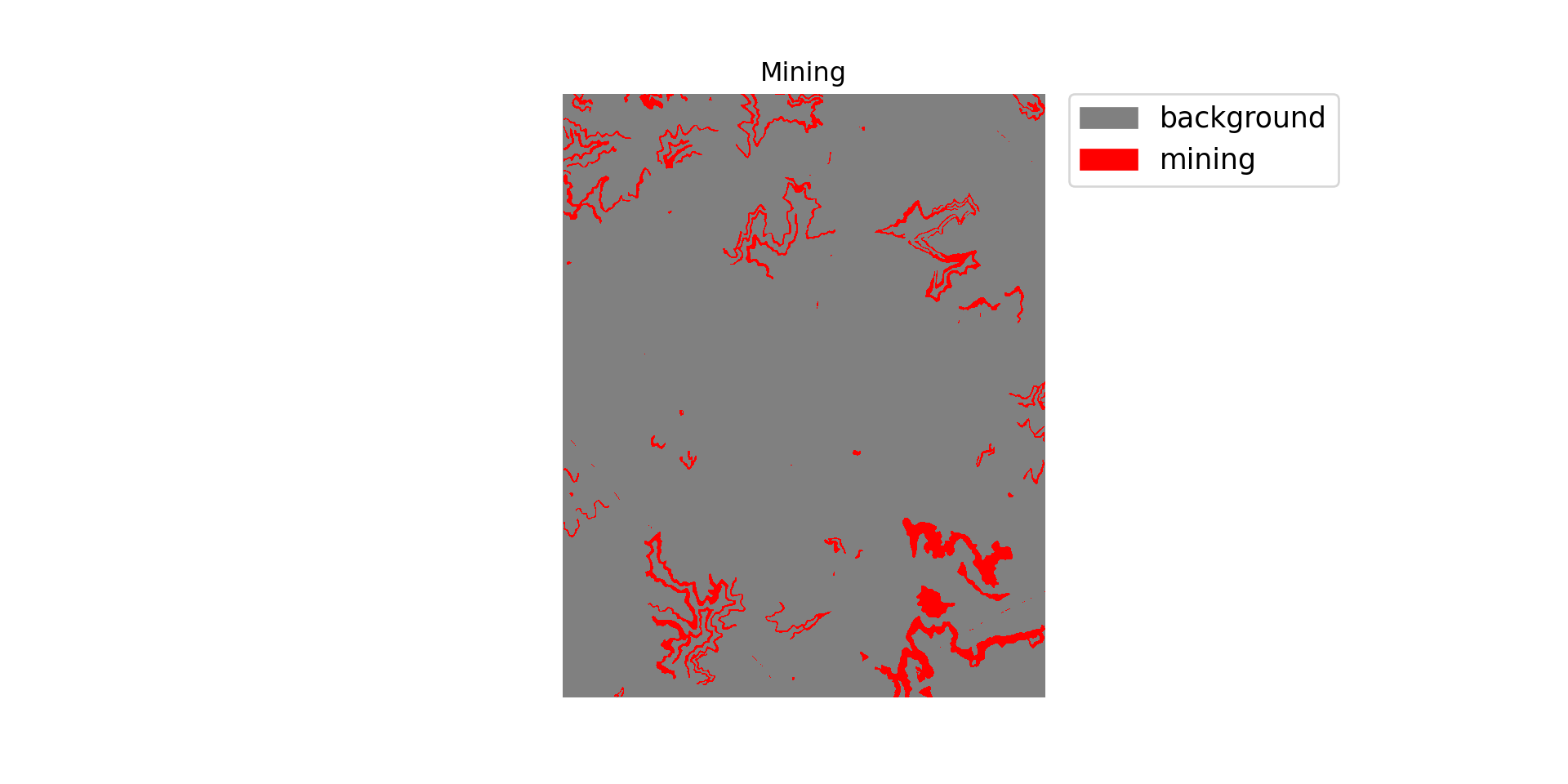

Using Variable Learning Rates

Before we end this module, I want to describe how to use different base learning rates for different components of the architecture. When using a pre-trained backbone as an encoder but not freezing the backbone during training, it has generally been suggested that using a lower learning rate for the encoder components relative to the decoder components and classification head can be beneficial. The idea here is that, since the encoder was initialized using non-random parameters, it will require less dramatic parameter updates in comparison to the decoder, which was initialized using random parameters. In my own experimentation and when using the same learning rate for all components of a model, I have generally struggled with unstable training processes when fine tuning a pre-trained encoder, as evident by loss and/or assessment metric results that vary greatly between epochs for the validation data. Using lower learning rates in the pre-trained but unfrozen encoder components has generally helped stabilize my training processes. In short, I highly recommend using variable learning rates for different components of the architecture if you are using pre-trained parameters.

Different learning rates can be implemented as follows:

1. Instantiate a model.
2. Build an array of dictionaries where each dictionary lists the parameters followed by the associated learning rate. If you are not sure how the modules are named, this can generally be determined by exploring the properties and classes associated with the instantiated model. In the example, I am using a learning rate of 1e-6 in the 1st and 2nd encoder blocks, a learning rate of 1e-5 in the 3rd and 4th encoder blocks, and a learning rate of 1e-4 in the decoder and classification head.

Once the array of dictionaries is defined, it can be passed to the optimizer during instantiation.

When using different learning rates, it is still possible to use optimizers that implement adaptive learning rates, such as RMSProp and Adam, momentum, weight decay, and learning rate schedulers. The stated learning rates just serve as a base learning rate but can still be augmented.

model = smp.Unet(
  encoder_name="resnet34", 
  encoder_weights="imagenet", 
  classes=5, 
  activation=None).to(device)

model_parameters = [
  {'params':model.encoder.layer1.parameters(), 'lr': 1e-6},
  {'params':model.encoder.layer2.parameters(), 'lr': 1e-6},
  {'params':model.encoder.layer3.parameters(), 'lr': 1e-5},
  {'params':model.encoder.layer4.parameters(), 'lr': 1e-5},
  {'params':model.decoder.parameters(), 'lr': 1e-4},
  {'params':model.segmentation_head.parameters(), 'lr': 1e-4}
  ] 

optimizer = torch.optim.AdamW(model_parameters)

Concluding Remarks

We highly encourage you to explore the Segmentation Models library. It offers an easy and intuitive means to implement a variety of semantic segmentation architectures and pre-trained CNN encoder backbones. In a later module and also using Segmentation Models, we will explore the use of a transformer-based encoder, SegFormer, for a UNet architecture.