Linear Regression with PyTorch
Linear Regression and Training Loops
Introduction
In this module, we will further explore neural networks and their implementation in PyTorch by implementing single linear regression. This module will also serve as an introduction to defining a loss metric and an optimization algorithm and how to properly set up a simple training loop.
OLS Linear Regression
We will begin with a review of linear regression. Below, I am importing numpy, pandas, seaborn, matplotlib, and statsmodels. We will use numpy for working with data arrays, pandas for working with data tables, and matplotlib and seaborn for graphing. We will implement ordinary least squares (OLS) linear regression using the statsmodels package.
For our experiments, we will use the mtcars dataset, which is provided as “cars.csv” in the provided class data. We will attempt to predict fuel efficiency in miles per gallon units using engine displacement. The data are read then represented as a pandas DataFrame.
import numpy as np
import pandas as pd
import seaborn as sns
import matplotlib.pyplot as plt
import statsmodels.api as sm
from statsmodels.graphics.regressionplots import abline_plot
cars = pd.read_csv("data/files/cars.csv")cars.head() mpg cylinders displacement ... model origin name
0 18.0 8 307.0 ... 70 1 chevrolet chevelle malibu
1 15.0 8 350.0 ... 70 1 buick skylark 320
2 18.0 8 318.0 ... 70 1 plymouth satellite
3 16.0 8 304.0 ... 70 1 amc rebel sst
4 17.0 8 302.0 ... 70 1 ford torino
[5 rows x 9 columns]Graphing displacement and mpg, it appears that there is a relationship between the variables: as expected, larger engine displacement generally correlates with reduced fuel efficiency. However, the relationship is not perfect. As a result, we would not expect to perfectly predict fuel efficiency using only engine displacement.
p1 = sns.scatterplot(x="displacement", y="mpg", data=cars)
plt.show(p1)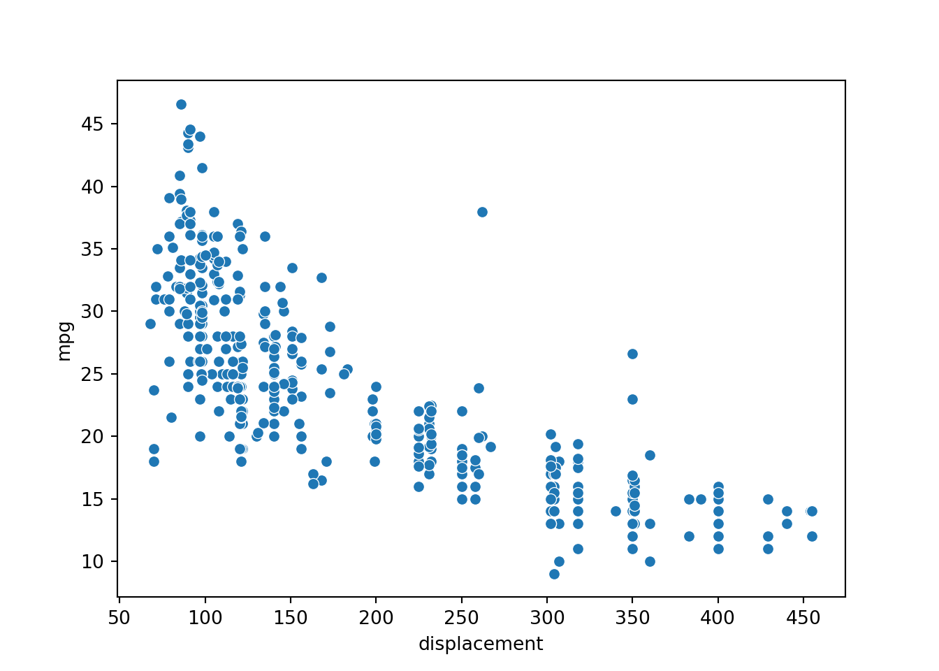
Let’s now fit a linear regression model using the ordinary least squares (OLS) method. OLS fits a linear regression model by attempting to minimize the square residuals. Using the statsmodels package, OLS linear regression is implemented as follows:
The x and y variables are extracted from the pandas DataFrame and converted to list objects.
I add a constant so that the y-intercept is included or estimated.
I fit the model using the fit() method.
I print the model summary.
The following relationship is predicted:
mpg = -0.0603*displacement + 35.1748
The R-squared for the model is 0.647, which suggests that ~65% of the variance in fuel efficiency is explained by engine displacement. A common next step would be to perform model diagnostics to make sure assumptions are not violated. However, I am only using this OLS linear regression output for comparison to the neural network implementation, so I will not worry about that here.
#https://www.geeksforgeeks.org/ordinary-least-squares-ols-using-statsmodels/
# Defining variables
x = cars['displacement'].tolist()
y = cars['mpg'].tolist()

# Add intercept
x = sm.add_constant(x)

# Fit
result = sm.OLS(y, x).fit()

# Print summary
print(result.summary())
OLS Regression Results
==============================================================================
Dep. Variable: y R-squared: 0.647
Model: OLS Adj. R-squared: 0.646
Method: Least Squares F-statistic: 725.0
Date: Tue, 16 Jul 2024 Prob (F-statistic): 1.66e-91
Time: 10:28:25 Log-Likelihood: -1175.5
No. Observations: 398 AIC: 2355.
Df Residuals: 396 BIC: 2363.
Df Model: 1
Covariance Type: nonrobust
==============================================================================
coef std err t P>|t| [0.025 0.975]
------------------------------------------------------------------------------
const 35.1748 0.492 71.519 0.000 34.208 36.142
x1 -0.0603 0.002 -26.926 0.000 -0.065 -0.056
==============================================================================
Omnibus: 41.373 Durbin-Watson: 0.919
Prob(Omnibus): 0.000 Jarque-Bera (JB): 60.024
Skew: 0.711 Prob(JB): 9.24e-14
Kurtosis: 4.264 Cond. No. 463.
==============================================================================
Notes:
[1] Standard Errors assume that the covariance matrix of the errors is correctly specified.#https://stackoverflow.com/questions/42261976/how-to-plot-statsmodels-linear-regression-ols-cleanly
ax = cars.plot(x='displacement', y='mpg', kind='scatter')
abline_plot(intercept=35.1748, slope=-0.0603, ax=ax)
plt.show()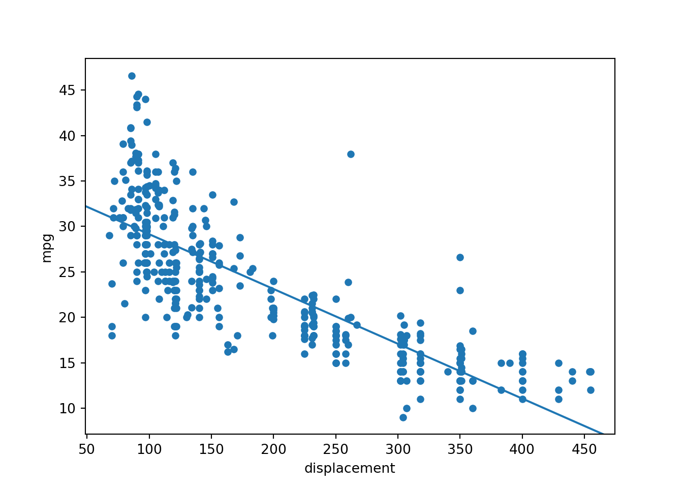
Linear Model with PyTorch
I am now ready to build a linear regression model using PyTorch. I begin by importing torch, torch.nn, and a specific function from the torch.autograd subpackage.
import torch
import torch.nn as nn
from torch.autograd import Variable
As with our fully connected neural network example from the first module, I must build the neural network by subclassing the PyTorch nn.Module class. The linear regression model is built as follows:
In the __init__() constructor method, parameters from the nn.Module parent or super class are inherited using super().__init__(). I also define a linear or fully connected layer using nn.Linear().
In the forward method, I specify that the input will pass through the linear layer, and the result will be returned.
That is it! This is pretty simple. However, how is this equivalent to single linear regression? Remember that a single node or neuron in a fully connected layer performs the following operation:
activation = weight*input + bias
In this case, the weight is equivalent to slope (m), and the bias is equivalent to the y-intercept (b). Since I am not using an activation function, such as a rectified linear unit (ReLU), following the linear layer, this is simply single linear regression.
class lmMod(nn.Module):
    def __init__(self):
        super().__init__()
        self.linear = torch.nn.Linear(1, 1)

    def forward(self, x):
        out = self.linear(x)
        return out
When using neural networks, it is generally a good idea to normalize the input data. This can be accomplished using the following equation:
(current value - mean value)/(standard deviation)
In the code blocks below, I calculate the mean and standard deviation of both the x and y variables. I then use these values to normalize the original data values.
x = np.array(cars['displacement'], dtype=np.float32)
x = x.reshape(-1, 1)
y = np.array(cars['mpg'], dtype=np.float32)
y = y.reshape(-1, 1)x.shape(398, 1)y.shape(398, 1)xMn = np.mean(x)
xSd = np.std(x)
yMn = np.mean(y)
ySd = np.std(y)
print(xMn), print(xSd), print(yMn), print(ySd)193.42587
104.13876
23.514572
7.806159
(None, None, None, None)xN = (x-xMn)/(xSd)
yN = (y-yMn)/(ySd)
print(np.mean(xN), np.std(xN), np.mean(yN), np.std(yN))5.7508e-08 1.0 9.5846666e-08 1.0This is a pretty simple, light-weight model, so I could train it on a CPU. However, I am going to use the GPU in this example. This requires checking to make sure a GPU is available. If a GPU is available, the device variable is set to “cuda:0”. If a GPU is not available, then the device is set to “cpu”.
device = torch.device("cuda:0" if torch.cuda.is_available() else "cpu")
print(device)cuda:0I next instantiate an instance of the model and move it to the defined device, in my case the GPU. I then define a learning rate and the number of epochs over which to iterate over the data during the learning process.
model = lmMod().to(device)modellmMod(
(linear): Linear(in_features=1, out_features=1, bias=True)
)lr = 0.01
epochs = 1000Since this is a regression problem, I will use the mean square error (MSE) loss. So, the parameter updates will be performed in an attempt to minimize the mean of the squared errors or residuals for the training data.
For the optimizer, I will use stochastic gradient descent (SGD). The torch.optim.SGD() function requires defining what the optimizer is optimizing, in this case the trainable model parameters, and the learning rate. There are only two trainable parameters in our simple neural network; the weight associated with the input displacement values and the bias are the only parameters that will be learned. Again, these correspond to the slope and y-intercept in the linear regression equation.
Remember that the learning rate specifies how much the weights or parameters will be adjusted with each update. Larger values indicate that the parameters can experience larger changes with each parameter update or optimization step.
criterion = torch.nn.MSELoss()
optimizer = torch.optim.SGD(model.parameters(), lr=lr)
I am now ready to train the model by iterating over the training data multiple times. The following are the general required steps in the training loop. Not setting up the training loop properly or defining the operations incorrectly or in the wrong order are common mistakes, so I will take some time to explain each component.
First, I need to read in both the predictor variables, in this case the normalized displacement values, and the targets, in this case the normalized mpg values. These data must also be moved to the device (the model and data must be on the same device in order to perform the training). Note that the methods used to read in data will vary by use case. For example, and as you will see in later modules, it is common to use a DataLoader object to read the data in mini-batches. Since this dataset is small, that is not necessary, so I am not making use of mini-batches.
The next step is to zero out the gradients. This is a very important step. You do not want the losses from prior iterations carrying over to the next iteration since each epoch should be an independent weight update. With the gradient cleared at the beginning of each iteration, you can then predict to the training data, calculate the loss, then use the computational graph and gradients to perform the back propagation and update the weights.
Next, I predict the training data using the defined model. This results in the output object.
Once predictions are made, I calculate the loss using the predictions and the target data.
In this example, I am saving the epoch number to a list object and the loss at each epoch to a different list. This is accomplished by initializing empty objects before beginning the training loop then appending the current epoch number and associated loss using the append() method for lists.
Once the data are predicted and the loss is calculated, the backpropagation is performed with the backward() method applied to the loss object. This calculates the gradients with respect to the parameters.
Finally, the model weights are updated using the optimizer via the step() method of the optimizer object. The learning rate, which was defined above, controls how much the parameters, in this case the single weight and bias, can change with each weight update or iteration.
There are some other components of the training loop that we will investigate in later modules. For example, to monitor the model’s performance when predicting to new data, to make sure it is generalizing, and to assess overfitting, it is best to use a separate validation set. Also, you may want to monitor other assessment metrics other than just the loss. Lastly, most training will be performed by feeding the data to the model in batches as opposed to all at once. This will require iterating over both the training epochs and the batches of data within each training epoch. Also, weight updates will commonly be performed after each batch as opposed to after each epoch. Again, you will see examples of these methods applied in later modules; however, this example demonstrates the basics of setting up a training loop.
lossLst = []
epochLst = []
for epoch in range(epochs+1):
    # Convert data to torch tensors and move to device
    inputs = Variable(torch.from_numpy(xN).to(device))
    labels = Variable(torch.from_numpy(yN).to(device))

    # Clear gradients
    optimizer.zero_grad()

    # Get outputs from the model
    outputs = model(inputs)

    # Get loss for the predicted output
    loss = criterion(outputs, labels)

    # Log loss and epoch number
    lossLst.append(loss.item())
    epochLst.append(epoch)

    # Get gradients w.r.t to parameters
    loss.backward()

    # Update parameters
    optimizer.step()

    # Print statement for every 50 epochs
    if epoch%50 == 0:
        print(f'Epoch: {epoch}, Loss: {loss.item():.4f}')
Epoch: 0, Loss: 1.2198
Epoch: 50, Loss: 0.4682
Epoch: 100, Loss: 0.3685
Epoch: 150, Loss: 0.3553
Epoch: 200, Loss: 0.3535
Epoch: 250, Loss: 0.3533
Epoch: 300, Loss: 0.3533
Epoch: 350, Loss: 0.3533
Epoch: 400, Loss: 0.3533
Epoch: 450, Loss: 0.3533
Epoch: 500, Loss: 0.3533
Epoch: 550, Loss: 0.3533
Epoch: 600, Loss: 0.3533
Epoch: 650, Loss: 0.3533
Epoch: 700, Loss: 0.3533
Epoch: 750, Loss: 0.3533
Epoch: 800, Loss: 0.3533
Epoch: 850, Loss: 0.3533
Epoch: 900, Loss: 0.3533
Epoch: 950, Loss: 0.3533
Epoch: 1000, Loss: 0.3533It is generally a good idea to assess how the loss changed as the model was trained over multiple epochs. To do so, I have combined my epoch and loss lists to a pandas DataFrame then used seaborn to plot the loss by epoch. As you can see, the loss leveled off before 200 epochs, which suggest that the model parameters were no longer updating or changing significantly. In other words, given the constraints of the single neuron with 1 associated weight and 1 associated bias, the optimal parameters that minimized the MSE loss were reached within 200 epochs. It was not possible to further reduce the model error or explain additional variance in mpg using the engine displacement variable.
resultDF = pd.DataFrame({'epoch':epochLst, 'loss':lossLst})
sp2 = sns.lineplot(data=resultDF, x="epoch", y="loss")
plt.show(sp2)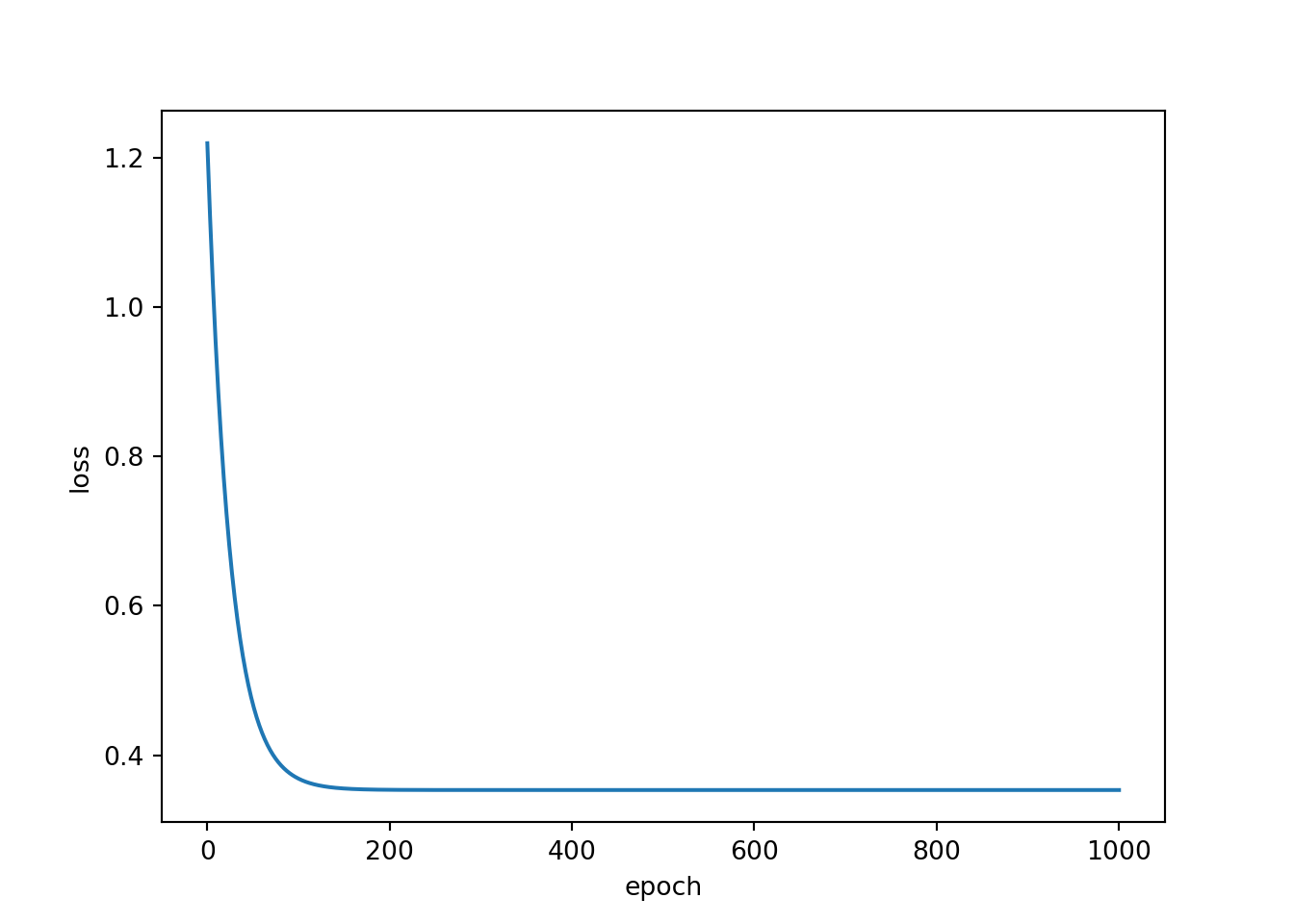
Explore the Impact of Learning Rate
In this section, we will explore how changing the learning rate impacts the loss. The model above used a learning rate of 0.01. Below, I have re-executed the model using learning rates of 0.001 and 0.0001. This requires that I re-instantiate the model, re-instantiate the loss criterion and optimizer, redefine the learning rate, redefine the empty loss and epoch lists, then re-execute the training loop. It is important to instantiate a new model and a new optimizer so that the training process starts over from a random initiation as opposed to from where it left off when training the prior model. This is another common mistake.
model = lmMod().to(device)
criterion = torch.nn.MSELoss()
lr = 0.001
optimizer = torch.optim.SGD(model.parameters(), lr=lr)
lossLst = []
epochLst = []
for epoch in range(epochs):
    inputs = Variable(torch.from_numpy(xN).to(device))
    labels = Variable(torch.from_numpy(yN).to(device))

    optimizer.zero_grad()

    outputs = model(inputs)

    loss = criterion(outputs, labels)

    lossLst.append(loss.item())
    epochLst.append(epoch)

    loss.backward()

    optimizer.step()
resultDF2 = pd.DataFrame({'epoch':epochLst, 'loss':lossLst})model = lmMod().to(device)
criterion = torch.nn.MSELoss()
lr = 0.0001
optimizer = torch.optim.SGD(model.parameters(), lr=lr)
lossLst = []
epochLst = []
for epoch in range(epochs):
inputs = Variable(torch.from_numpy(xN).to(device))
labels = Variable(torch.from_numpy(yN).to(device))
optimizer.zero_grad()
outputs = model(inputs)
loss = criterion(outputs, labels)
lossLst.append(loss.item())
epochLst.append(epoch)
loss.backward()
optimizer.step()resultDF3 = pd.DataFrame({'epoch':epochLst, 'loss':lossLst})Now that I have ran all three models using the three different learning rates, I next add the associated learning rate to each DataFrame then combine the DataFrames to a single object. I also have to reset the row indices due to repeats. Next, I use seaborn to plot the loss by epoch for each separate model.
This result clearly shows the impact of changing the learning rate. When using a smaller learning rate, weight updates with each epoch or optimization step is much smaller. Thus, it would take more epochs to train the model. The results indicate that 0.01 is a better learning rate for this model than the other two rates tested. The learning rate is generally an important setting. We will discuss choosing a learning rate in more detail in later modules.
resultDF["lr"] = "0.01"
resultDF2["lr"] = "0.001"
resultDF3["lr"] = "0.0001"
resultAll = pd.concat([resultDF, resultDF2, resultDF3])
resultAll.reset_index(inplace=True)
sns.lineplot(data=resultAll, x="epoch", y="loss", hue="lr")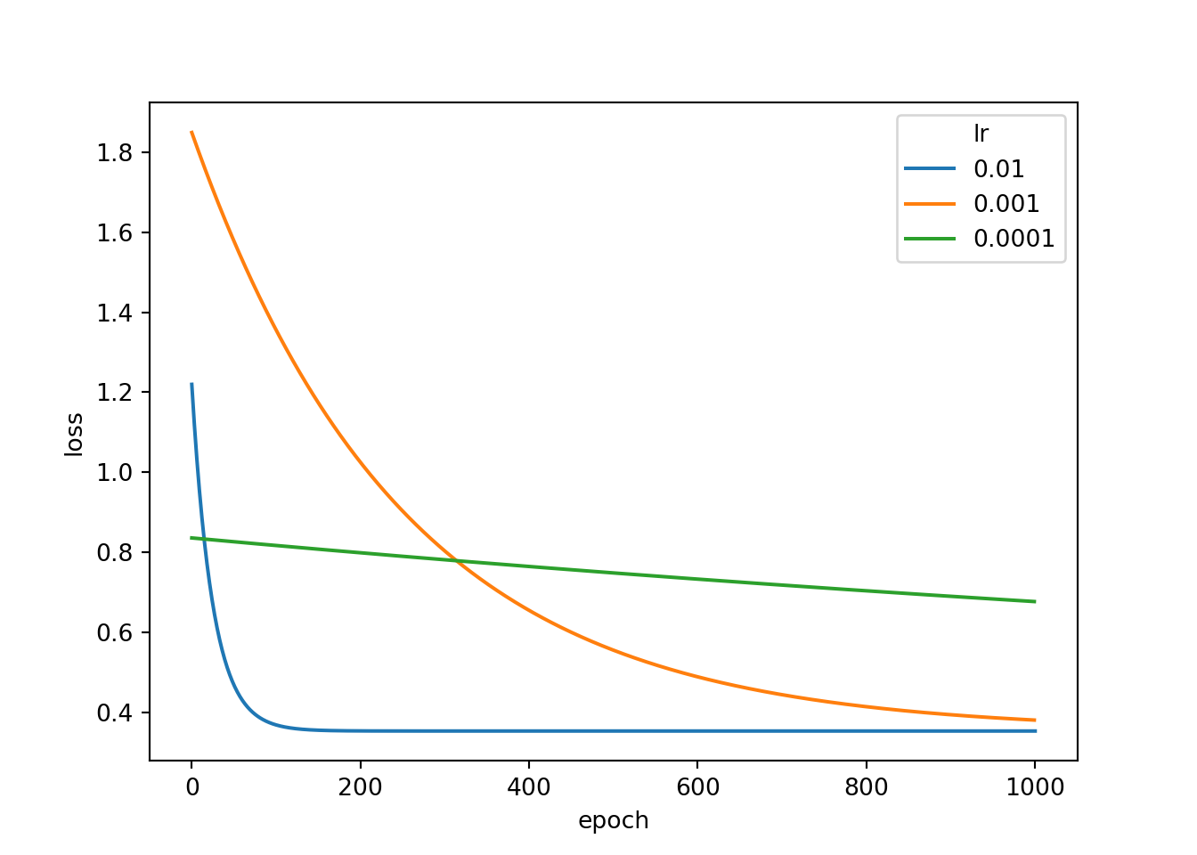
Comparison to OLS Regression
To end this module, let’s compare our OLS linear regression model with the neural network model. Below, I have re-instantiated the model then re-trained it using a learning rate of 0.01. I then use the trained model to predict back to the displacement data. The result is then detached, moved to the CPU, converted to a numpy array, then flattened to a 1D array. Remember that I normalized both the displacement and mpg data prior to training the model. In order to obtain the fuel efficiency predictions in the correct units, I need to multiply them by the standard deviation and add the mean that was calculated for the mpg variable above.
Next, I re-run the OLS model and use it to predict back to the displacement data.
model = lmMod().to(device)
criterion = torch.nn.MSELoss()
lr = 0.01
optimizer = torch.optim.SGD(model.parameters(), lr=lr)
lossLst = []
epochLst = []
for epoch in range(epochs):
    inputs = Variable(torch.from_numpy(xN).to(device))
    labels = Variable(torch.from_numpy(yN).to(device))

    optimizer.zero_grad()

    outputs = model(inputs)

    loss = criterion(outputs, labels)

    lossLst.append(loss.item())
    epochLst.append(epoch)

    loss.backward()

    optimizer.step()
predNN = model(Variable(torch.from_numpy(xN).cuda())).detach().cpu().numpy().flatten()
predNN = (predNN*ySd)+yMnx = cars['displacement'].tolist()
y = cars['mpg'].tolist()
x = sm.add_constant(x)
result = sm.OLS(y, x).fit()predOLS = result.predict(x)In order to make graphs, I then combine the original mpg and displacement variables with the predicted mpg from the neural network and OLS models into a new DataFrame. I then use matplotlib and seaborn to graph the results.
The resulting models, represented by the lines in the graphs, seem to be the same or very similar.
compareDF = pd.DataFrame({'mpg': cars['mpg'].to_numpy(), 'displacement': cars['displacement'].to_numpy(), 'mpgNN': predNN, 'mpgOLS': predOLS})compareDF.head() mpg displacement mpgNN mpgOLS
0 18.0 307.0 16.668064 16.668052
1 15.0 350.0 14.075926 14.075908
2 18.0 318.0 16.004959 16.004945
3 16.0 304.0 16.848911 16.848899
4 17.0 302.0 16.969475 16.969464fig, ax = plt.subplots(1,2)
sns.lineplot(data=compareDF, x="displacement", y="mpgNN", ax=ax[0])
sns.scatterplot(data=compareDF, x="displacement", y="mpg", ax=ax[0])
sns.lineplot(data=compareDF, x="displacement", y="mpgOLS", ax=ax[1])
sns.scatterplot(data=compareDF, x="displacement", y="mpg", ax=ax[1])
plt.show(fig)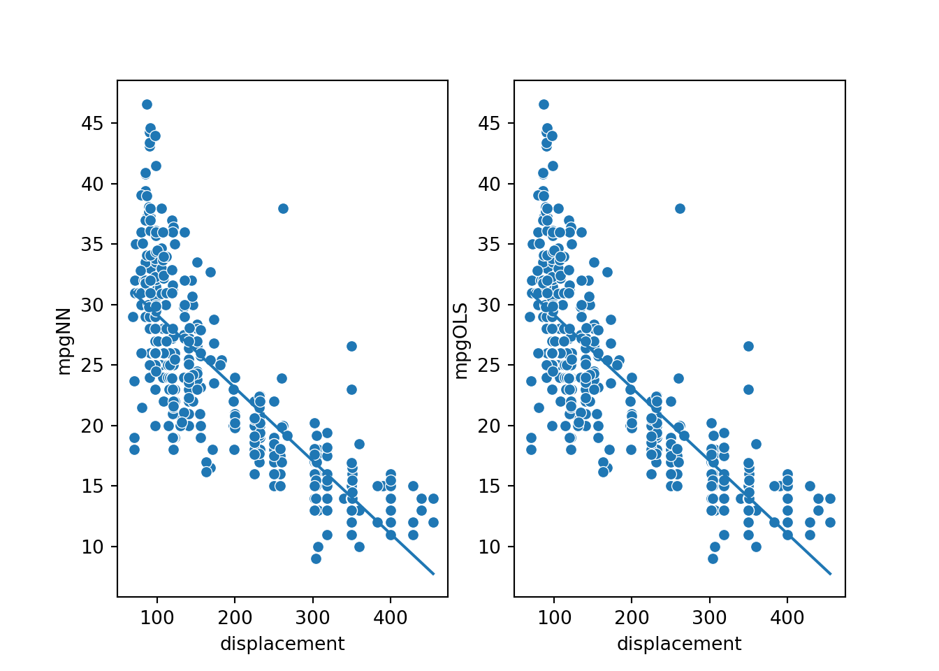
To test whether the two models have the same parameters (slope and y-intercept), I calculate the slope using two of the data points. The result is -0.0603, which is equivalent to the OLS slope, ignoring rounding error. Next, I calculate the y-intercept using a data point and by subtracting the displacement multiplied by the slope from the associated mpg prediction. The result is 35.175, which is again the same as the result for the OLS model, ignoring rounding error.
# Slope = (y2-y1)/(x2-x1)
slopeNN = (compareDF['mpgNN'].iloc[2]-compareDF['mpgNN'].iloc[1])/(compareDF['displacement'].iloc[2]-compareDF['displacement'].iloc[1])
slopeNN-0.06028228998184204# b = y - mx
bNN = compareDF['mpgNN'].iloc[2]-(compareDF['displacement'].iloc[2]*slopeNN)
bNN35.17472732067108I obtained the same results using the OLS method and via training the neural network using stochastic gradient descent and the MSE loss. Does this make sense? The OLS algorithm attempts to minimize the sum of squared residuals between the actual and predicted values using the partial derivative of the cost function, in this case MSE, with respect to the coefficients of determination, setting the partial derivatives equal to zero, then solving for each of the coefficients: the slope and y-intercept.
OLS attempts to find the slope and y-intercept that minimize the MSE, and this is accomplished using the method described above. The stochastic gradient descent optimizer attempts to minimize the loss, in this case MSE, by incrementally changing the model weights over multiple training epochs and using the gradient of the loss with respect to the model parameters. So, in both cases the goal is the same: find the parameters that minimize the loss. However, the means to accomplish this is different. As a result, it makes sense that these methods would yield the same final model.
Unfortunately, the OLS method cannot be generalized to estimate parameters that will minimize the loss for all neural network architectures. In contrast, SGD and its derivatives, are more generalizable. Thus, they are currently used as the primary means to update model parameters during the learning process.
Concluding Remarks
The goal of this section was to introduce you to the process of training a neural network by implementing simple linear regression using a neural network and comparing the results obtained to those from OLS regression. In the next module, we will explore loss and assessment metrics in greater detail.