DataSets and DataLoaders

Introduction

We have one last topic to cover before we can train a fully connected neural network. You can now define a network architecture; specify loss functions, assessment metrics, and optimizers; and build a simple training loop. Key missing pieces are loading in data, converting them into tensors, and defining batches. Before we begin, it should be noted that the PyTorch package updates regularly, and data handling is one component that has tended to change significantly between releases. For example, a beta library, called TorchData, is in development that is specifically focused on data loading and handling. Here, I will demonstrate using the DataSet and DataLoader classes made available in torch.utils. For working with imagery data specifically, torchvision provides custom dataset classes that are subclasses of DataSet including DatasetFolder, ImageFolder, and VisionDataset. There are also datasets built into torchvision. Please see this page for more details: https://pytorch.org/vision/stable/datasets.html.

As already discussed, tensors are a flexible data model that can represent a wide variety of data types. For example, tabulated data can be represented as a 2D array in which each row represents a sample and each column stores different information about each record. An image can be stored as a 3D array (Channels, Height, and Width) while a video can be stored as a 4D array (Time/Frame, Channels, Height, and Width).

Raw data can exist in many forms and be stored in a variety of file formats. For example, an image can be stored as a TIFF, JPEG, or PNG file. Images can also vary based on their radiometric gain (i.e., 8-bit, 11-bit, or 16-bit) and the number of channels. Given these complexities, we need a flexible means by which to be able to read files and convert them to tensors of the appropriate data types and shapes for input to the deep learning process. This is the purpose of the DataSet and DataLoader classes in PyTorch.

As normal, I begin by importing the required packages. Since I will be working with arrays and data tables, I import numpy and pandas. I will use the pyplot subpackage of the matplotlib package to visualize image data. I will need to work with file paths and file names, so I import os. As in the Losses and Assessment Metrics module, I will use scikit-learn to recode differentiated classes from strings to numeric codes. The torch package and torch.nn subpackage are imported. The DataSet class is available in the utils.data.dataset subpackage while the DataLoader class is available in torch.utils.data.

We will be working with satellite data in this module, so I import the rasterio package with an alias of rio. I have found that this package can sometimes be tricky to install into an environment with a lot of other packages. Please consult the package documentation if you are having issues. Lastly, I will use earthpy to visualize the satellite data.

Since I will be working with images, it is a good idea to use the GPU as opposed to CPU. Since I will not be training a model in this module, only preparing the data, DataSet, and DataLoader, this is not strictly necessary. However, it will be preferable in the next module when I train and evaluate a model.

import numpy as np
import pandas as pd
import matplotlib
from matplotlib import pyplot as plt 

import os

from sklearn import preprocessing 

import torch
import torch.nn as nn
from torch.utils.data.dataset import Dataset
from torch.utils.data import DataLoader

import rasterio as rio
import earthpy as et
import earthpy.spatial as es
import earthpy.plot as ep

device = torch.device("cuda:0" if torch.cuda.is_available() else "cpu")
print(device)

cuda:0

EuroSatAllBands Dataset

In this class, we will make use of the EuroSat dataset, which can be downloaded from Kaggle: https://www.kaggle.com/datasets/apollo2506/eurosat-dataset. There are two versions of these data: EuroSat and EuroSatAllBands. We will make use of the data with all 13 bands: EuroSatAllBands. The band designations are as follows:

1 = Coastal Aerosol (60 m)
2 = Blue (10 m)
3 = Green (10 m)
4 = Red (10 m)
5 = Red Edge 1 (20 m)
6 = Red Edge 2 (20 m)
7 = Red Edge 3 (20 m)
8 = Near Infrared (NIR) (10 m)
8a = NIR Narrow (10 m)
9 = Water Vapor (60 m)
10 = Cirrus Cloud (60 m)
11 = Shortwave Infrared (SWIR) 1 (20 m)
12 = SWIR 2 (20 m)

These data were derived from the Multispectral Instrument (MSI) onboard the Sentinel-2A and 2B satellites, which are operated by the European Space Agency (ESA) as part of the Copernicus Program. The bands vary by spatial resolution from 10 m to 60 m; however, all bands have been resampled to a 10 m spatial resolution in the EuroSat and EuroSatAllBands datasets. We will only use the bands that were originally collected at 10 m or 20 m in this course: red, green, blue, red edge 1, red edge 2, red edge 3, NIR, narrow NIR, SWIR 1, and SWIR 2. This paper introduces these data:

Helber, P., Bischke, B., Dengel, A. and Borth, D., 2019. Eurosat: A novel dataset and deep learning benchmark for land use and land cover classification. IEEE Journal of Selected Topics in Applied Earth Observations and Remote Sensing, 12(7), pp.2217-2226.

To follow along with this example, you will need to download the data from Kaggle and uncompress the folder. Note that this is a fairly large dataset, so it will take some time to download and uncompress.

Data Preparation

In this first section, we will focus on some data preparation steps. You will need to set the path to your copy of the uncompressed data. I first list all of the subfolders inside of the EuroSatallBands folder. Each subfolder stores images representing different classes: annual crop, forest, herbaceous vegetation, highways, industrial, pasture, permanent crop, residential, river, and sea/lake. There is a total of 10 classes differentiated. In the first code block, I am using the os package and list comprehension to list all of the folders. I then subset out only the base name from the entire folder path.

In the next code block, I create an empty DataFrame then loop through all of the subfolders to list all of the files that they contain. I create list objects that store the file name, the full file path, and the class name, which is the same as the subfolder in which it occurs. I then combine these into a DataFrame and merge them into the initially empty imgDF DataFrame.

PyTorch requires that each category be represented with a numeric code as opposed to a string. So, as you already saw in the Losses and Assessment Metrics module, I use the LabelEncoder() function from the preprocessing subpackage of scikit-learn to generate numeric codes for each class, which are defined alphabetically. I then write this to a new column in the imgDF DataFrame. As a result, I now have a DataFrame in which each row represents a sample image and discrete columns provide the file name, full file path, class name, and class numeric code.

Lastly, I print the imgDF object to make sure it looks correct. There are a total of 27,597 samples in the dataset.

folder = "C:/myFiles/work/dl/eurosat/EuroSATallBands/"
clsLst = [ f.path for f in os.scandir(folder) if f.is_dir() ]
clsLst = [os.path.basename(f) for f in clsLst]
clsLst

['AnnualCrop', 'Forest', 'HerbaceousVegetation', 'Highway', 'Industrial', 'Pasture', 'PermanentCrop', 'Residential', 'River', 'SeaLake']

imgDF = pd.DataFrame(columns = ["file", "fullpath", "class"])
for f in clsLst:
    currentFolder = folder + f + "/"
    currentClass = f
    imgLst = os.listdir(currentFolder)
    pathLst = [currentFolder+img for img in imgLst]
    imgDFCurrent = pd.DataFrame({"file": imgLst, "fullpath":pathLst})
    imgDFCurrent["class"] = f
    imgDF = pd.concat([imgDF, imgDFCurrent], axis=0, ignore_index = True)

label_encoder = preprocessing.LabelEncoder()
imgDF['code'] = label_encoder.fit_transform(imgDF['class'])

imgDF.head()

                  file  ... code
0     AnnualCrop_1.tif  ...    0
1    AnnualCrop_10.tif  ...    0
2   AnnualCrop_100.tif  ...    0
3  AnnualCrop_1000.tif  ...    0
4  AnnualCrop_1001.tif  ...    0

[5 rows x 4 columns]

The EuroSatAllBands dataset comes with CSV files that list out the images into separate training, testing, and validation sets. However, we will step through the process of defining these data partitions on our own since you may need to do this with your own datasets.

I first shuffle the rows of the DataFrame using the sample() pandas method. Setting the frac parameter to 1 means that all rows will be maintained, so I am not drawing a sample from the dataset but simply shuffling it. This is done to avoid any autocorrelation in the data.

I then print the number of rows or samples per class using pandas. It doesn’t appear as if there is any issues with data imbalance, so I will not worry about this specific issue in my analyses. In other words, there are an ample number of samples in each class.

imgDF = imgDF.sample(frac = 1)

print(imgDF.groupby('class').size())

class
AnnualCrop              3000
Forest                  3000
HerbaceousVegetation    3000
Highway                 2500
Industrial              2500
Pasture                 2000
PermanentCrop           2500
Residential             3000
River                   2500
SeaLake                 3597
dtype: int64

Next, I split the data using a stratified random sampling method. This involves first splitting out a training set then further splitting the remaining samples into separate testing and validation sets. Although stratified random sampling is not really necessary here, I wanted to demonstrate this since it is common to want to apply stratification to your sampling. Here, I have used 60% of the data for training, 20% for testing, and 20% for validation. Remember that the training data are used to train the model and guide the parameter updates while the validation data are used to assess the model at the end of each training epoch. The test data are reserved to assess the final model. Printing the lengths of each DataFrame, you can see that there are 16,558 training, 5,519 validation, and 5,520 testing samples.

Since I want to save these data partitions and tables for later use, such as in the next module when I actually train a neural network, I write them to disk as CSV files using the to_csv() method from pandas. I then read the results back into the workflow.

train = imgDF.groupby('class', group_keys=False).apply(lambda x: x.sample(frac=0.6))
leftovers=imgDF.drop(train.index)
test=leftovers.groupby('class', group_keys=False).apply(lambda x: x.sample(frac=0.5))
val=leftovers.drop(test.index)

train.to_csv(folder+"mytrain.csv", index=False)
test.to_csv(folder+"mytest.csv", index=False)
val.to_csv(folder+"myval.csv", index=False)

train = pd.read_csv(folder+"mytrain.csv")
test = pd.read_csv(folder+"mytest.csv")
val = pd.read_csv(folder+"myval.csv")

train.head()

                  file  ... code
0    AnnualCrop_83.tif  ...    0
1  AnnualCrop_2451.tif  ...    0
2  AnnualCrop_2955.tif  ...    0
3   AnnualCrop_179.tif  ...    0
4  AnnualCrop_1906.tif  ...    0

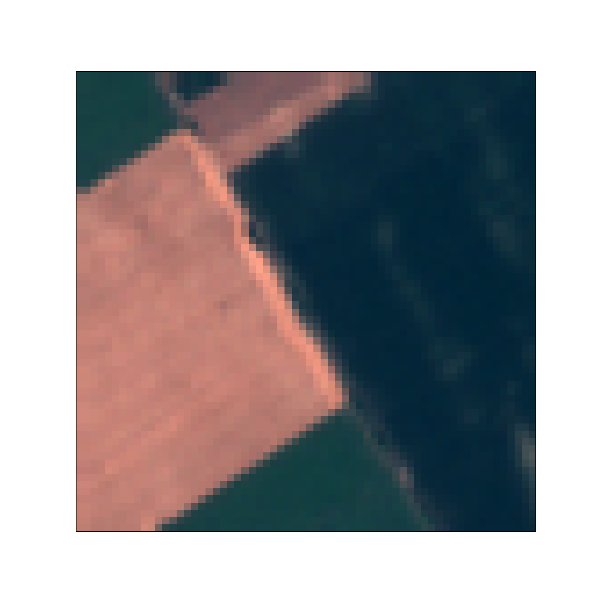
[5 rows x 4 columns]

Before moving on, let’s plot one of the images as a check. To plot the image, I extract one of the image paths from the train object. I then use the rasterio package to read the image. When using rasterio, you need to open a connection to the image, read the image in as a numpy array using read(), and then close the connection to the image. If you open a connection to an image with rasterio, you should also remember to close it. The read() function also allows you to only read in a subset of the available bands if desired.

I next print the array shape and calculate the channel means using np.mean and aggregating across the height and width dimensions. Note that rasterio, similar to PyTorch, uses the channels-first convention, as opposed to the channels-last convention. The array has a shape of (13,64,64). So, there are 13 channels, and each image chip has a height and width of 64 pixels. Since the pixel size is 10 m, this would be equivalent to spatial dimensions of 640 m by 640 m.

Lastly, I use the plot_rgb() function from earthpy to plot a simulated true color composite of the image. The red channel shows red, the green channel shows green, and the blue channel shows blue.

img1 = train.iloc[0,1]
source = rio.open(img1)
img1Arr = source.read()
source.close()

print(img1Arr.shape)

(13, 64, 64)

print(np.mean(img1Arr, axis=(1,2)))

[1451.07348633 1301.21630859 1310.90039062 1690.94335938 1882.68334961
 2300.97167969 2693.98120117 2679.53027344  674.34667969   14.05541992
 2567.92431641 1461.91552734 3229.57080078]

ep.plot_rgb(
    img1Arr,
    rgb=(3,2,1), # place the combination of rgb
)

print(train.iloc[0,2])

AnnualCrop

Aggregate to Band Means

When we start working with convolutional neural networks (CNNs) we will use the actual images as input to the model. However, for our fully connected neural network examples, we will use the band means. It is possible to use all of the pixels, which requires flattening the data. However, this would result in a large input space (13 bands by 64 rows by 64 columns). This would be one way to work with these data using a fully connected architecture. However, to reduce the size of the data, I will aggregate to obtain band means. This mimics a traditional, pixel-based image classification that does not incorporate spatial patterns or image context information. Again, we will use spatial context information and the full set of pixels when we investigate convolutional neural networks.

In the first code block, I aggregate the pixel data for each image chip to obtain band means. This requires (1) defining an empty DataFrame to write to, (2) reading a file path, (3) reading the data in as a numpy array using rasterio, (4) subsetting out the 10 bands that I want to include in the analysis, (5) calculating the band means by aggregating all of the pixels by channel, and (6) writing the results to the DataFrame. This process is completed for the training, validation, and testing data separately to obtain three separate DataFrames. Note that this code may take some time to execute given the large number of images that must be processed.

Printing the trainAgg result as an example, you can see that I now have a table in which each row represents an image and the following information is stored: class, class numeric code, and band means for the 10 bands of interest. Next, I use the describe() method to further explore the results and obtain summary statistics for each band.

trainAgg = pd.DataFrame(columns=["class", "code", "blue", "green", 
"red", "red_edge1", "red_edge2", 
"red_edge3", "NIR", "NIR_Narrow", "swir1", "swir2"])
for i in range(0, len(train)):
    img1 = train.iloc[i,1]
    source = rio.open(img1)
    img1Arr = source.read()
    source.close()
    img1Arr = img1Arr[[1,2,3,4,5,6,7,8,11,12], :, :]
    img1Mns = np.mean(img1Arr, axis=(1,2))
    trainAgg2 = pd.DataFrame({"class": [train.iloc[i,2]], 
    "code": [train.iloc[i,3]], 
    "blue":[img1Mns[0]],
    "green":[img1Mns[1]],
    "red":[img1Mns[2]], 
    "red_edge1":[img1Mns[3]], 
    "red_edge2":[img1Mns[4]], 
    "red_edge3":[img1Mns[5]], 
    "NIR":[img1Mns[6]], 
    "NIR_Narrow":[img1Mns[7]], 
    "swir1":[img1Mns[8]], 
    "swir2":[img1Mns[9]]})
    trainAgg = pd.concat([trainAgg, trainAgg2], axis=0, ignore_index=True)

testAgg = pd.DataFrame(columns=["class", "code", "blue", "green", 
"red", "red_edge1", "red_edge2", 
"red_edge3", "NIR", "NIR_Narrow", "swir1", "swir2"])
for i in range(0, len(test)):
    img1 = test.iloc[i,1]
    source = rio.open(img1)
    img1Arr = source.read()
    source.close()
    img1Arr = img1Arr[[1,2,3,4,5,6,7,8,11,12], :, :]
    img1Mns = np.mean(img1Arr, axis=(1,2))
    testAgg2 = pd.DataFrame({"class": [test.iloc[i,2]], 
    "code": [test.iloc[i,3]], 
    "blue":[img1Mns[0]],
    "green":[img1Mns[1]],
    "red":[img1Mns[2]], 
    "red_edge1":[img1Mns[3]], 
    "red_edge2":[img1Mns[4]], 
    "red_edge3":[img1Mns[5]], 
    "NIR":[img1Mns[6]], 
    "NIR_Narrow":[img1Mns[7]], 
    "swir1":[img1Mns[8]], 
    "swir2":[img1Mns[9]]})
    testAgg = pd.concat([testAgg, testAgg2], axis=0, ignore_index=True)

valAgg = pd.DataFrame(columns=["class", "code", "blue", "green", 
"red", "red_edge1", "red_edge2", 
"red_edge3", "NIR", "NIR_Narrow", "swir1", "swir2"])
for i in range(0, len(val)):
    img1 = val.iloc[i,1]
    source = rio.open(img1)
    img1Arr = source.read()
    source.close()
    img1Arr = img1Arr[[1,2,3,4,5,6,7,8,11,12], :, :]
    img1Mns = np.mean(img1Arr, axis=(1,2))
    valAgg2 = pd.DataFrame({"class": [val.iloc[i,2]], 
    "code": [val.iloc[i,3]], 
    "blue":[img1Mns[0]],
    "green":[img1Mns[1]],
    "red":[img1Mns[2]], 
    "red_edge1":[img1Mns[3]], 
    "red_edge2":[img1Mns[4]], 
    "red_edge3":[img1Mns[5]], 
    "NIR":[img1Mns[6]], 
    "NIR_Narrow":[img1Mns[7]], 
    "swir1":[img1Mns[8]], 
    "swir2":[img1Mns[9]]})
    valAgg = pd.concat([valAgg, valAgg2], axis=0, ignore_index=True)

trainAgg.head()

        class code         blue  ...  NIR_Narrow        swir1        swir2
0  AnnualCrop    0  1301.216309  ...  674.346680  1461.915527  3229.570801
1  AnnualCrop    0  1042.024902  ...  758.629395  1189.456543  2714.708008
2  AnnualCrop    0  1411.484619  ...  761.717041  1621.122070  3900.247314
3  AnnualCrop    0  1188.903809  ...  638.532471  1469.149170  3986.078125
4  AnnualCrop    0  1313.136719  ...  948.018066  1656.648682  3609.164551

[5 rows x 12 columns]

trainAgg.describe()

               blue         green  ...         swir1         swir2
count  16558.000000  16558.000000  ...  16558.000000  16558.000000
mean    1116.076457   1035.312140  ...   1103.833501   2552.017877
std      255.543289    312.298762  ...    670.886884   1120.899907
min      606.409912    399.506836  ...      6.082764     86.967773
25%      917.461609    827.478638  ...    599.183594   2110.309570
50%     1082.943848    996.796997  ...   1080.136963   2713.484741
75%     1279.106201   1222.766968  ...   1542.290955   3275.200439
max     2356.135010   2479.513184  ...   3394.176514   5837.482422

[8 rows x 10 columns]

Since we will use these aggregated data in the next module, I save them to disk as CSV files then read them back into the workflow as pandas DataFrames. I will also want to be able to normalize these data before providing them to the fully connected neural network. This can be accomplished using the following equation to obtain a z-score:

(current value - mean)/standard deviation

In order to accomplish this, I need to have the band means and standard deviations calculated. This is accomplished in the last code block were the columns associated with the band means are extracted, the mean or standard deviation is calculated for each band, and the results are flattened to a 1D numpy array.

trainAgg.to_csv(folder + "train_aggregated.csv")
testAgg.to_csv(folder + "test_aggregated.csv")
valAgg.to_csv(folder + "val_aggregated.csv")

trainAgg = pd.read_csv(folder + "train_aggregated.csv")
testAgg = pd.read_csv(folder + "test_aggregated.csv")
valAgg = pd.read_csv(folder + "val_aggregated.csv")

trainAggMns = np.array(trainAgg.iloc[:,3:].mean(axis=0)).flatten()
print(trainAggMns)

[1116.07645724 1035.31213955  937.87729602 1184.29159721 1971.09456594
 2334.38145703 2262.04021603  724.95266414 1103.83350066 2552.01787743]

trainAggSDs = np.array(trainAgg.iloc[:,3:].std(axis=0)).flatten()
print(trainAggSDs)

[ 255.54328897  312.29876238  479.85770488  500.93361557  779.66575883
  976.84613356  970.08515215  384.49257895  670.88688372 1120.89990655]

Pixel-Level Statistics

In this section, we will explore calculating band means and standard deviations at the pixel-level per band as opposed to using the aggregated data, as demonstrated above. Pixel-level band means and standard deviations are necessary or useful for normalizing data. Although we will not use this information when working with fully connected neural networks, we will use it later once we start exploring convolutional neural networks. Since the data volume is now much larger, as a result of working with pixels as opposed to the aggregated data, this can be accomplished using batches. So, this will be the first time that we need to define a DataSet and DataLoader.

A custom DataSet is created by subclassing the DataSet class. The goal of a DataSet is to generate a pipeline that delivers to the DataLoader and training loop tensors of the correct shape and data type for each sample. The __getitem__() method defines how a single sample is read then converted into a tensor. The other required method is __len__(), which returns the number of available samples. Let’s now step through this first DataSet subclass.

Within the __init__() constructor method, I inherit from the parent or super class using super().__init__. I then define new parameters. In this case, the DataSet will only accept a DataFrame object.

Within the __getitem__() method, I (1) get the file path from the associated DataFrame column, (2) get the class numeric code from the associated DataFrame column and convert it to a numpy array, (3) read the image in as a numpy array using rasterio (making sure to close the connection after reading the data), (4) convert the image data type to 32-bit float, (5) subset out the 10 bands of interest, (6) convert the label and image numpy arrays to torch tensors using the from_numpy() function (I must also squeeze and flatten the data so that they are the correct shape), (7) convert the label tensor to a long integer data type, and (8) return the image and label tensors. Note that the idx variable references the current row or image being processed. It is important that the __getitem__() method return torch tensors for both the predictor variables, in this case the multiband image, and the labels with the shapes and data types required by the neural network architecture.

Inside of the __getitem__() method, it is common to perform data transformations on arrays representing image data, such as cropping, resampling, and normalization. Additional transformations can be randomly applied to augment the data and to potentially combat overfitting. The torchvision package provides functions for applying data transformations. We will not explore those here, but will do so when we define DataSets for training CNNs in later modules. For semantic segmentation, we will specifically use the albumentations package.

The __len__() method simply returns the number of available samples, which in this case is the length or number of rows in the input DataFrame.

class EuroSat(Dataset):
    
    def __init__(self, df):
        super().__init__
        self.df = df
    
    def __getitem__(self, idx):
        image_name = self.df.iloc[idx, 1]
        label = self.df.iloc[idx, 3]
        label = np.array(label)
        source = rio.open(image_name)
        image = source.read()
        source.close()
        image = image.astype('float32')
        image = image[[1,2,3,4,5,6,7,8,11,12], :, :]
        image = torch.from_numpy(image)
        label = torch.from_numpy(label)
        label = label.long()
        return image, label 
        
    def __len__(self):
        return len(self.df)

Once a DataSet subclass is defined, an instance can be instantiated. Here, I am creating an instance of the DataSet called trainDS, which represents the training dataset specifically. Calling len() on the dataset returns the number of training samples, in this case 16,558.

trainDS = EuroSat(train)
print(len(trainDS))

This DataSet is too large to read in all samples at once. Instead, samples will need to be read in using batches. Weight updates will be performed after predicting to each batch, calculating the loss, and performing backpropagation. The number of samples that can be read in at once will depend on several factors including the complexity of the neural network architecture, the available resources (e.g., GPU VRAM and number of GPUs), and the size of the images (e.g., you could read in more 64 by 64 pixel chips than 512 by 512 pixel chips). In order to define these data batches, I will need to create a DataLoader.

Below, I am generating a DataLoader from the trainDS dataset. The batch size is 32, the data will be randomly reshuffled at each learning epoch, and the data will not be subsampled at each epoch. The number of workers argument specifies how many subprocesses to use while loading data. At the time of this writing, I have had issues using more than one worker within the Windows operating system. So, I have set this to 0, which is the default. This does seem to work fine on Linux-based machines. The pin_memory option is used to copy tensors into the pinned device or CUDA memory before returning them. The drop_last argument is used to drop the last batch from the computation if it is an incomplete batch or if the total number of samples is not evenly divisible by the batch size.

trainDL = torch.utils.data.DataLoader(trainDS, batch_size=32, shuffle=True, sampler=None,
num_workers=0, pin_memory=False, drop_last=False)

Now that I have a DataSet and a DataLoader defined and instantiated, I define a function that loops over the batches to calculate the mean and standard deviation of the bands at the pixel-level. This function was obtained from the provided link. I then run this function on the DataLoader object. The result is a set of band means and standard deviations as 1D tensors. Again, these values can be useful for normalizing the data.

When you have separate training, testing, and validation sets, it is common to calculate the band means and standard deviations from the training data only but then apply these values to all three DataSets to perform the normalization. This is so that all of the DataSets will have a similar distribution and also to avoid a data leak, in which the model learns something about the testing and/or validation data, which is not desired if we aim to assess overfitting and generalization. Sometimes data will be normalized using means and standard deviations from another dataset. This is especially common when using transfer learning since we want the input data to have a distribution that is similar to that of the data used to train the original model.

#https://www.binarystudy.com/2021/04/how-to-calculate-mean-standard-deviation-images-pytorch.html
def batch_mean_and_sd(loader, inChn):
    
    cnt = 0
    fst_moment = torch.empty(inChn)
    snd_moment = torch.empty(inChn)

    for images, _ in loader:
        b, c, h, w = images.shape
        nb_pixels = b * h * w
        sum_ = torch.sum(images, dim=[0, 2, 3])
        sum_of_square = torch.sum(images ** 2,
                                  dim=[0, 2, 3])
        fst_moment = (cnt * fst_moment + sum_) / (cnt + nb_pixels)
        snd_moment = (cnt * snd_moment + sum_of_square) / (cnt + nb_pixels)
        cnt += nb_pixels

    mean, std = fst_moment, torch.sqrt(snd_moment - fst_moment ** 2)        
    return mean,std

band_stats = batch_mean_and_sd(trainDL, 10)

band_stats

(tensor([1116.0757, 1035.3129,  937.8776, 1184.2919, 1971.0939, 2334.3823,
        2262.0425,  724.9523, 1103.8335, 2552.0176]), tensor([ 331.1133,  396.2515,  594.6111,  574.7384,  885.5202, 1114.8973,
        1144.0782,  406.0714,  768.5239, 1268.6659]))

DataSet and DataLoader for Tabulated Data

To further explore defining a DataSet and using a DataLoader, we will now define and prepare them for the fully connected neural network use case in which the predictor variables will be the mean channel values calculated from all the image pixels, and the dependent variable will be the class, as represented with a numeric code. In this new DataSet subclass the resulting tensors for each sample should be the normalized mean channel values for each band while the dependent variable should be the class code.

This new DataSet subclass requires three parameters: an input DataFrame and the band means and standard deviations for normalization. These are defined inside of the __init__() constructor method. Inside of the __getitem__() method, I (1) read in the columns representing the band means and the column representing the class code from the input DataFrame, (2) convert the band means to a numpy array, (3) normalize the band values using the band means and standard deviations to obtain a z-score, (4) convert the label to a numpy array, (5) convert the normalized band means to a 32-bit float data type, (6) convert the bands to a torch tensor using the from_numpy() method (I must also remove a dimension with squeeze() and convert the data to a float type), and (6) convert the labels to a torch tensor and change the data type to a long integer. This method returns the bands and label tensors.

Again, the __len__() method must return the number of samples.

class EuroSat(Dataset):
    
    def __init__(self, df, bndMns, bndSDs):
        super().__init__
        self.df = df
        self.bndMns = bndMns
        self.bndSDs = bndSDs
    
    def __getitem__(self, idx):
        bands = [self.df.iloc[idx, 3:]]
        label = [self.df.iloc[idx, 2]]
        bands = np.array(bands)
        bands = (bands-self.bndMns)/self.bndSDs
        label = np.array(label)
        bands = bands.astype('float32')
        bands = torch.from_numpy(bands).squeeze().float()
        label = torch.from_numpy(label).squeeze().float()
        label = label.long()
        return bands, label 
        
    def __len__(self):
        return len(self.df)

Next, I instantiate an instance of the EuroSat Dataset subclass called trainDS. This requires three inputs: the DataFrame of aggregated band means and class codes and the aggregated channel means and standard deviations. The means and standard deviations are used to perform data normalization.

Next, I instantiate the DataLoader using the dataset object. I use a batch size of 128. Since I am now only using the band means as opposed to the entire image, I should be able to use more samples per batch.

trainDS = EuroSat(trainAgg, trainAggMns, trainAggSDs)

trainDL = torch.utils.data.DataLoader(trainDS, batch_size=128, shuffle=True, sampler=None,
num_workers=0, pin_memory=False, drop_last=False)

Once you have instantiated the DataLoader, it is generally a good idea to explore it to make sure that the results are as expected. To do so, I generate an example batch of data using the next() and iter() functions. I then unpack the resulting object to obtain separate bands and labels objects.

The shape of the bands object is (128, 10). This makes sense since the batch size is 128 and the number of channels is 10. The labels have a shape of (128), which makes sense since there is one label for each of the 128 samples in the batch. The data type for the bands is 32-bit float while the data type for the labels is long integer. Generally, PyTorch will expect 32-bit float values for the predictor variables. The required data type for the labels will vary by problem type. For a multiclass classification, a long integer data type is generally expected.

Extracting out a single image from the batch, you can see that the bands object consists of a 1D array of band means that have been normalized while the label is a single value.

So, it looks like the DataLoader is providing data by batch in the expected format. We will make use of this DataLoader in the next module when we train a fully connected neural network.

batch = next(iter(trainDL))
bands, labels = batch
print(f'Batch Image Shape: {bands.shape}, Batch Label Shape: {labels.shape}')

Batch Image Shape: torch.Size([128, 10]), Batch Label Shape: torch.Size([128])

print(f'Batch Image Data Type: {bands.dtype}, Batch Label Data Type: {labels.dtype}')

Batch Image Data Type: torch.float32, Batch Label Data Type: torch.int64

testBands = bands[1]
testLabel = labels[1]
print(testBands)

tensor([3.0204, 2.9572, 2.9141, 2.5920, 1.2392, 0.9345, 0.8765, 0.0636, 2.6624,
        0.8827])

print(testLabel)

tensor(0)

DataSet and DataLoader for Image Data

In this last section, we will generate another DataSet and DataLoader. This is the DataLoader that we will use in the CNN examples in later modules. However, I will make some modifications to allow for transformations to be applied. In comparison to the above example, this DataLoader will return images and labels as opposed to band means and labels.

We will now be returning back to using the DataFrame in which each row represents an image and contains the file name, file path, class name, and class numeric code. We will also make use of the pixel-level band means and standard deviations calculated above to perform normalization.

Our new DataSet subclass will accept a DataFrame and pixel-level band means and standard deviations in order to perform normalization. These are defined inside of the __init__() constructor method. Inside of the __getitem__() method, I (1) extract the file path from the DataFrame, (2) extract the numeric label from the DataFrame, (3) read the image chip as a numpy array using rasterio (again, remember to close the connection to the file once it is read), (4) subset out the required bands, (5) perform normalization using the provided pixel-level band means and standard deviations, (6) convert the image to a 32-bit float data type, (7) convert the image and labels to tensors using the from_numpy() function, and (8) convert the label to a long integer data type. This function returns a processed image and associated label as tensors. Again, the __len__() method returns the number of samples.

class EuroSat(Dataset):
    
    def __init__(self, df, mnImg, sdImg):
        self.df = df
        self.mnImg = mnImg
        self.sdImg = sdImg
    
    def __getitem__(self, idx):
        image_name = self.df.iloc[idx, 1]
        label = self.df.iloc[idx, 3]
        label = np.array(label)
        source = rio.open(image_name)
        image = source.read()
        source.close()
        image = image[[1,2,3,4,5,6,7,8,11,12], :, :]
        image = np.subtract(image, self.mnImg)
        image = np.divide(image, self.sdImg)
        image = image.astype('float32')
        image = torch.from_numpy(image)
        label = torch.from_numpy(label)
        label = label.long()
        return image, label 
        
    def __len__(self):
        return len(self.df)

Before instantiating an instance of the EuroSat dataset, I must prepare the channel mean and standard deviation data. I first convert the data to list objects. These lists are then processed to create tensors of shape (10, 64, 64) in which each channel holds the mean or standard deviation for that channel (all values will be the same in each pixel within each channel). This is so that the shape of these tensors match that of the image to which they will be applied. Once these tensors are obtained, I can instantiate the DataSet.

bndMns = np.array(band_stats[0].tolist())
bndSDs = np.array(band_stats[1].tolist())

mnImg = np.repeat(bndMns[0], 64*64).reshape((64,64,1))
for b in range(1,len(bndMns)):
    mnImg2 = np.repeat(bndMns[b], 64*64).reshape((64,64,1))
    mnImg = np.dstack([mnImg, mnImg2])
mnImg = np.transpose(mnImg, (2,0,1))

sdImg = np.repeat(bndSDs[0], 64*64).reshape((64,64,1))
for b in range(1,len(bndSDs)):
    sdImg2 = np.repeat(bndSDs[b], 64*64).reshape((64,64,1))
    sdImg = np.dstack([sdImg, sdImg2])
sdImg = np.transpose(sdImg, (2,0,1))

print(mnImg.shape)

(10, 64, 64)

print(sdImg.shape)

(10, 64, 64)

trainDS = EuroSat(train, mnImg, sdImg)

In the DataLoader, I have set the batch_size parameter back to 32 since I will now be loading in (10,64,64) image chips as opposed to the pixel-level band means.

trainDL = torch.utils.data.DataLoader(trainDS, batch_size=32, shuffle=True, 
num_workers=0, pin_memory=False, drop_last=True)

Again, it is good to check data batches to make sure there are no issues. The shape of my batches is as expected (32,10,64,64). The label batch consists of 32 single values. The data types for the image values is 32-bit float while the labels are long integers. The pixel values appear to be normalized.

Looking at a single image, you can see that the shape is (10,64,64) while the label is a single value. The range of codes seem correct and the pixel values appear to be normalized.

batch = next(iter(trainDL))
images, labels = batch
print(f'Batch Image Shape: {images.shape}, Batch Label Shape: {labels.shape}')

Batch Image Shape: torch.Size([32, 10, 64, 64]), Batch Label Shape: torch.Size([32])

print(f'Batch Image Data Type: {images.dtype}, Batch Label Data Type: {labels.dtype}')

Batch Image Data Type: torch.float32, Batch Label Data Type: torch.int64

print(f'Batch Image Band Means: {torch.mean(images, dim=(0,2,3))}')

Batch Image Band Means: tensor([ 0.0477,  0.0187,  0.0194, -0.0287, -0.0159, -0.0089, -0.0257, -0.1359,
         0.0593, -0.0332])

print(f'Batch Label Minimum: {torch.min(labels, dim=0)}, Batch Label Maximum: {torch.max(labels, dim=0)}')

Batch Label Minimum: torch.return_types.min(
values=tensor(0),
indices=tensor(9)), Batch Label Maximum: torch.return_types.max(
values=tensor(9),
indices=tensor(5))

testImg = images[1]
testMsk = labels[1]
print(f'Image Shape: {testImg.shape}, Label Shape: {testMsk.shape}')

Image Shape: torch.Size([10, 64, 64]), Label Shape: torch.Size([])

print(f'Image Data Type: {testImg.dtype}, Label Data Type: {testMsk.dtype}')

Image Data Type: torch.float32, Label Data Type: torch.int64

Since we now have image data as opposed to tables, it would make sense to actually visualize a batch of images and associated labels. This is accomplished using the code below. First, I create a function to display a single image. This requires (1) unnormalizing the image using the band means and standard deviations, (2) subsetting out the bands that will be displayed, (3) changing the dimension order to channels-last since this is expected by matplotlib, and (4) rescaling the data and converting them to an 8-bit unsigned data type.

I also define a dictionary to map the class codes back to the class names.

I then build the figure using matplotlib. This involves (1) initializing a plot with 32 subplots, (2) looping through the data to map an image to each subplot, and (3) assigning a title to each subplot that is the class label. The image is displayed using the imshow() method from matplotlib. I am using the red, green, and blue channels here, so the result will be a simulated true color composite.

If you are using a similar method to display image data and the images look too dark, too bright, or have too high or too low contrast, you may need to experiment with the scaling and normalization parameters.

def img_display(img, mnImg, sdImg):
    img = np.multiply(img, sdImg)
    img = np.add(img, mnImg)
    image_vis = img[[2,1,0],:,:]
    image_vis = image_vis.permute(1,2,0)
    image_vis = (image_vis.numpy()/6000)*255
    image_vis = image_vis.astype('uint8')
    return image_vis

dataiter = iter(trainDL)
images, labels = next(dataiter)
cover_types = {0: 'Ann Crop', 
1: 'Forest', 
2: 'Herb Veg', 
3: 'Highway', 
4: 'Industrial',
5: 'Pasture',
6: 'Perm Crop',
7: 'Residential',
8: 'River',
9: 'SeaLake'}

fig, axis = plt.subplots(4, 8, figsize=(15, 10))
for i, ax in enumerate(axis.flat):
    with torch.no_grad():
        image, label = images[i], labels[i]
        ax.imshow(img_display(image, mnImg, sdImg))
        ax.set(title = f"{cover_types[label.item()]}") 
plt.show()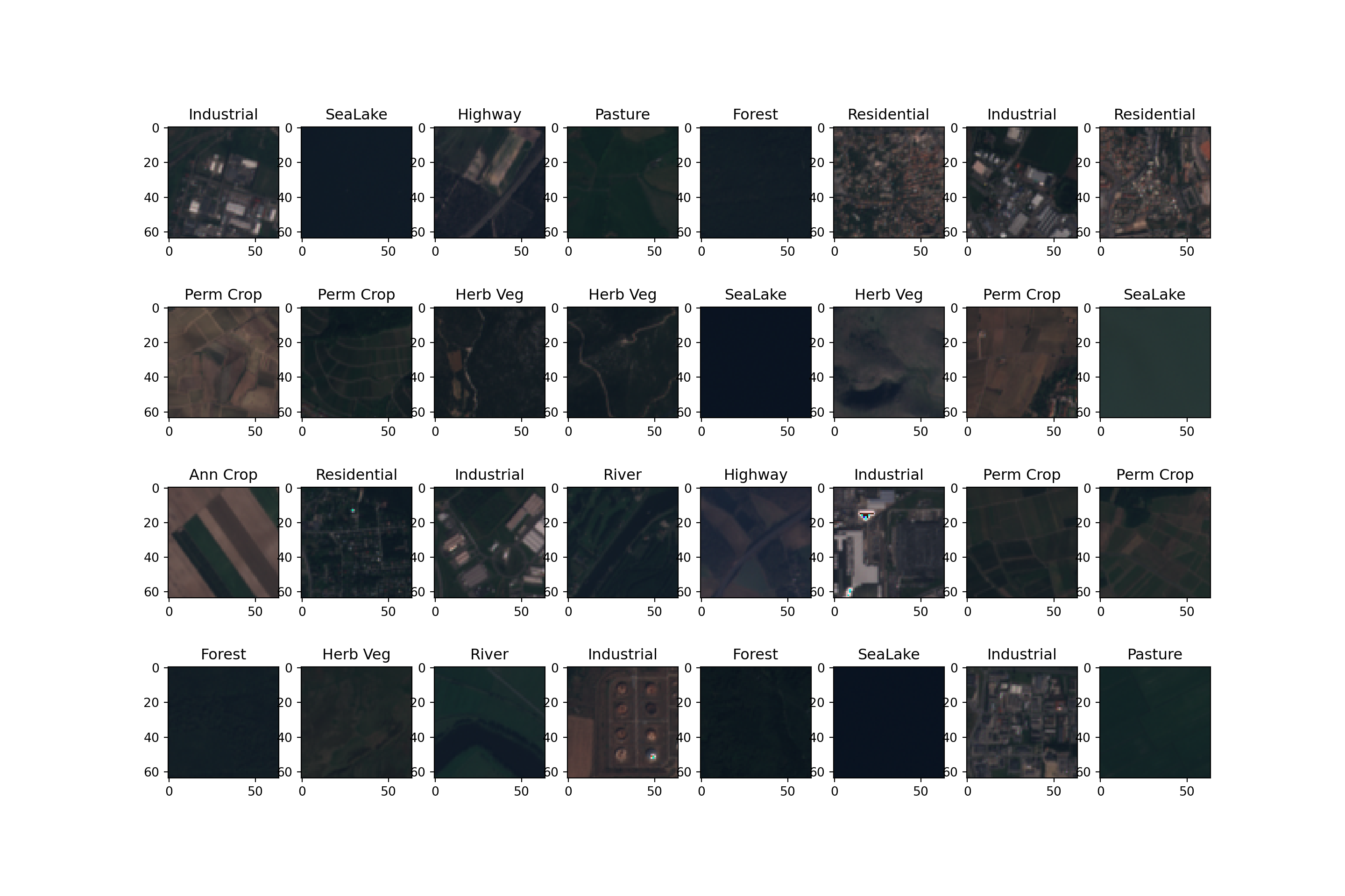

Concluding Remarks

The primary purpose of this module was to serve as an introduction to preparing data and using the DataSet and DataLoader PyTorch classes. Again, this component of PyTorch seems to update rapidly, so you may need to consult the documentation to adjust code to match current workflows. Also, it is possible to load data without using the DataSet and DataLoader classes. If so, your methods would need to be able to generate tensors for each sample of the correct shape and data type and deliver the data to the training loop in batches. However, I find that it is easiest to subclass or use the DataSet and DataLoader classes and advise against trying to build a pipeline from scratch unless you are experienced with PyTorch.

I did want to note a few tips associated with using DataSets and DataLoaders since I have found this to be one of the trickier components of the workflow.

In this module I used rasterio to read image data. I did this because the images were generated using geospatial data and are multispectral, or have more than three bands. When you just have three-band or grayscale data, you can load images using other packages, such as PIL or cv2. I generally prefer to use cv2 over PIL, but this is just personal preference.
When loading images into numpy arrays or tensors using different packages, they may not adhere to the same conventions. For example, some packages may use the channels-first convention while others use the channels-last convention. PyTorch expects the channels-first convention. Dimensions can be reordered using the numpy transpose() function or the PyTorch permute() function.
PyTorch can be picky about data types. However, you can convert between data types pretty easily using numpy or PyTorch, such as converting 32-bit float data to long integer or unsigned 8-bit data to 32-bit float. Error messages are generally helpful when troubleshooting data type issues.
It is generally good practice to assess your data batches to make sure the output is in the correct shape, the data types have been defined correctly, and the dimension ordering is correct.
If working with images, it is good to plot the images and the associated labels.
Normalization is a common pre-processing requirement. Calculating means and standard deviations are sometimes necessary to apply normalization. When using transfer learning, you may normalize using the means and standard deviations from the original dataset as opposed to the current dataset. These values can generally be looked up. For example, the ImageNet means and standard deviations are as follows: means = [0.485, 0.456, 0.406] and standard deviations = [0.229, 0.224, 0.225]. In order to normalize to a range of 0 to 1, it is common to use a mean of 0.5 and a standard deviation of 0.5.
Be careful not to cause a data leak. For example, you should normalize data using a common mean and standard deviation, such as those for ImageNet, or a mean of 0.5 and a standard deviation of 0.5. Normalizing the testing and validation data using their own means and standard deviations may result in inconsistent distributions between the dataset or a data leak by allowing the algorithm information about the distribution of the withheld data.
Data transformations may also be applied to either prepare the data (e.g., crop, resample, or normalize) or augment the data to combat overfitting. There are functions available within torchvision to accomplish this. We will explore this in later modules. We will also explore the albumentations package for applying transformations when undertaking semantic segmentation.
You may need to experiment with batch sizes to efficiently use your hardware while also not running out of RAM or VRAM.
Using more than one GPU can greatly improve training time and allow for larger data batches. We will discuss how to use multiple GPUs in a later module.
I have generally found that loading images from a magnetic hard drive can be much slower than loading them from a solid-state drive. Thus, I recommend storing your data on a solid-state drive, at least while conducting training, validation, and inference.
In this module, I focused on reading files from disk by listing their names, file paths, and associated labels in a pandas DataFrame. I did this because I have found this method to be intuitive. However, there are other means to load data that do not require listing each sample in a DataFrame. Please consult the PyTorch and torchvision documentation for examples of other dataset generation and data loading methods.

Now that we have covered defining fully connected architectures, loss metrics, assessment metrics, optimizers, training loops, DataSets, and DataLoaders, we are ready to train and assess a model. In the next section, we will train and assess a fully connected neural network to predict or differentiate land cover classes using the band means calculated from the pixels within each image chip. We will also incorporate validation at the end of each training epoch and an assessment of the final model using the withheld testing dataset.