import numpy as np
import pandas as pd
import matplotlib
from matplotlib import pyplot as plt
import seaborn as sns
plt.rcParams['figure.figsize'] = [20, 20]

import os

from sklearn import preprocessing
from sklearn.metrics import confusion_matrix
from sklearn.metrics import classification_report


import torch
import torch.nn as nn
from torch.utils.data.dataset import Dataset
from torch.utils.data import DataLoader

import torchmetrics as tm

import tqdm as notebook_tmTrain a Fully Connected Neural Network
Train a Fully Connected Neural Network
Introduction
You are now ready to bring together what you have been learning in the prior modules to train a fully connected neural network. For this example, we will use the band means that we calculated in the prior module for the EuroSat data to predict the associated land cover class. Note that this is not the intended use of these data; the data are meant to be analyzed using all pixel values or the entire image as opposed to band means. However, only using band means will greatly reduce the training time. Also, I feel that this is a valuable exercise as this mimics a traditional pixel-based classification in which spatial context is not considered.
For the first part of this module, I will keep my explanations brief since we have already discussed these components in the prior modules. Instead, we will focus on the back-matter where the model is trained using a training loop and then assessed with the withheld data.
Prepare Data
In this first section, the goal is to prepare the data, and I am just re-executing code that I created in prior modules. First, I read in the required packages. There is nothing new here other than calling in some specific functions from scikit-learn, which I will use for model validation. I also set the device variable to the GPU. Again, this greatly speeds up training, validation, and inference.
device = torch.device("cuda:0" if torch.cuda.is_available() else "cpu")
print(device)cuda:0I then call in the tables that I generated in the prior module that contain the band means, class names, and class numeric codes. Remember that the EuroSatAllBands dataset already has defined training, validation, and testing splits. However, we created our own in order to learn how this is accomplished.
Next, I re-execute code from the last module to obtain the training data band means and standard deviations. These will be used to normalize the data. Remember that it is generally best practice to normalize all the data partitions using either (1) the same normalization parameters (such as setting each band mean to 0.5 and the standard deviation to 0.5), (2) normalization parameters from another dataset if transfer learning is used, or (3) parameters obtained from just the training data. Again, this is to avoid a data leak and also to make sure all data partitions have a similar distribution.
#Read in CSV files
folder = "C:/datasets/archive/EuroSATallBands/"
trainAgg = pd.read_csv(folder + "train_aggregated.csv")
testAgg = pd.read_csv(folder + "test_aggregated.csv")
valAgg = pd.read_csv(folder + "val_aggregated.csv")
trainAgg.head() Unnamed: 0 class code ... NIR_Narrow swir1 swir2
0 0 AnnualCrop 0 ... 605.556396 1268.607910 3924.330566
1 1 AnnualCrop 0 ... 841.336670 2405.725830 3024.959473
2 2 AnnualCrop 0 ... 884.121094 2339.997070 3115.421631
3 3 AnnualCrop 0 ... 697.208008 2102.330566 2547.223145
4 4 AnnualCrop 0 ... 861.247070 1752.863770 3029.635742
[5 rows x 13 columns]trainAggMns = np.array(trainAgg.iloc[:,3:].mean(axis=0)).flatten()
print(trainAggMns)[1115.38296803 1032.78632781 934.42367534 1179.63372106 1965.45598147
2328.46128297 2256.31645472 723.06439937 1096.76794609 2545.5668783 ]trainAggSDs = np.array(trainAgg.iloc[:,3:].std(axis=0)).flatten()
print(trainAggSDs)[ 255.37392552 312.41467923 480.85890988 503.13822569 781.83525125
979.84301129 972.96770341 384.01325659 668.86946005 1124.41850788]I next define a subclass of the DataSet class. This was the second DataSet subclass that we created in the last module. Remember that the DataSet subclass must have a __getitem__() method defined that returns the predictor values and target labels for an individual sample in the format expected by the neural network architecture. The __len__() method must return the number of samples. Please consult the prior module for the details as to how this specific DataSet subclass was defined.
class EuroSat(Dataset):

    def __init__(self, df, bndMns, bndSDs):
        super().__init__
        self.df = df
        self.bndMns = bndMns
        self.bndSDs = bndSDs

    def __getitem__(self, idx):
        bands = [self.df.iloc[idx, 3:]]
        label = [self.df.iloc[idx, 2]]
        bands = np.array(bands)
        bands = (bands-self.bndMns)/self.bndSDs
        label = np.array(label)
        bands = bands.astype('float32')
        bands = torch.from_numpy(bands).squeeze().float()
        label = torch.from_numpy(label).squeeze().float()
        label = label.long()
        return bands, label

    def __len__(self):
        return len(self.df)
Next, I instantiate three DataSets using the EuroSat class: trainDS, valDS, and testDS. Again, these will be used to train the model, assess the model performance at the end of each training epoch, and assess the final model, respectively. The network will only learn from the training data while the validation and test data will be used to assess performance, generalization, and overfitting.
After the datasets are instantiated, I define DataLoaders. I am using a mini-batch size of 256 since each record consists of only the 10 band means and the associated target class. If I were using the entire 64 by 64 pixel image chips, this batch size would likely be too large and I would run out of memory unless I had access to a GPU with lots of VRAM or multiple GPUs. Again, you may need to adjust this batch size if you are running this code depending on your system specifications.
trainDS = EuroSat(trainAgg, trainAggMns, trainAggSDs)
testDS = EuroSat(testAgg, trainAggMns, trainAggSDs)
valDS = EuroSat(valAgg, trainAggMns, trainAggSDs)
trainDL = torch.utils.data.DataLoader(trainDS, batch_size=256, shuffle=True, sampler=None,
num_workers=0, pin_memory=False, drop_last=False)
testDL = torch.utils.data.DataLoader(testDS, batch_size=256, shuffle=True, sampler=None,
num_workers=0, pin_memory=False, drop_last=False)
valDL = torch.utils.data.DataLoader(valDS, batch_size=256, shuffle=True, sampler=None,
num_workers=0, pin_memory=False, drop_last=False)Lastly, I perform some checks to make sure the DataSet and DataLoader are returning the data in the correct format. You can see that each batch consists of a tensor with shape (256, 10), which houses the predictor variables, and a tensor with shape (256), which houses the class numeric codes. The first dimension is the batch or sample dimension. For the predictor variable tensor, the second dimension is the variable dimension. The labels could be stored with a shape (256, 1); however, the network expects a 1D tensor.
The predictor variables have a data type of 32-bit float while the labels have a data type of 64-bit integer (i.e., long integer). Again, this is expected by the network. When calling a single image from the mini-batch, we can see that it consists of a 1D array of band values and a single value representing the numeric code of the class label. Again, the data have been normalized to z-scores using the training data means and standard deviations.
batch = next(iter(trainDL))
bands, labels = batch
print(f'Batch Image Shape: {bands.shape}, Batch Label Shape: {labels.shape}')
Batch Image Shape: torch.Size([256, 10]), Batch Label Shape: torch.Size([256])print(f'Batch Image Data Type: {bands.dtype}, Batch Label Data Type: {labels.dtype}')Batch Image Data Type: torch.float32, Batch Label Data Type: torch.int64testBands = bands[1]
testLabel = labels[1]
print(testBands)tensor([-0.3399, -0.1202, 0.0323, 0.3726, 0.1750, 0.0297, 0.1628, 1.7696,
0.8964, 0.0800])print(testLabel)tensor(2)Data Visualization
Before training the model, let’s visualize the distribution of each spectral band by class. This is accomplished using grouped boxplots, which are generated using matplotlib and seaborn. I generate a plot with multiple axes or subplots then fill each with data for a specific spectral band. I am using the training data table, so the values are not normalized yet. I also rename the x-axis labels and rotate them a bit to make them more legible.
There are a few notable patterns here. First, there seems to be some common patterns between the bands. For example, the three visible bands tend to have similar trends, suggesting that these variables are correlated. Also, there is generally overlap of the interquartile range (IQR) for many of the classes for many of the bands. This indicates that this may not be a simple problem to solve since the spectral signatures of some of the classes may not be that different from each other. However, it does appear that some of the bands offer differentiation of specific classes. For example, the sea/lake class has low spectral reflectance in the NIR and SWIR bands. The pasture class seems to have high spectral reflectance in some of the red edge, NIR, and SWIR bands.
Again, it is generally a good idea to explore your data using summary statistics and/or visualizations prior to implementing the training process to better understand the data and to potentially flag any errors or issues with the dataset or processing pipeline.
fig, axs = plt.subplots(5,2)
fig.set_size_inches(18.5, 10.5)
sns.boxplot(ax=axs[0,0], data=testAgg, x="class", y="blue")
sns.boxplot(ax=axs[0,1], data=testAgg, x="class", y="green")
sns.boxplot(ax=axs[1,0], data=testAgg, x="class", y="red")
sns.boxplot(ax=axs[1,1], data=testAgg, x="class", y="red_edge1")
sns.boxplot(ax=axs[2,0], data=testAgg, x="class", y="red_edge2")
sns.boxplot(ax=axs[2,1], data=testAgg, x="class", y="red_edge3")
sns.boxplot(ax=axs[3,0], data=testAgg, x="class", y="NIR")
sns.boxplot(ax=axs[3,1], data=testAgg, x="class", y="NIR_Narrow")
sns.boxplot(ax=axs[4,0], data=testAgg, x="class", y="swir1")
sns.boxplot(ax=axs[4,1], data=testAgg, x="class", y="swir2")
for r in range(0,5):
    axs[r,0].set_xticklabels(["Annual Crop", "Forest", "Grass", "Highway",
"Industrial", "Pasture", "Permanent Crop", "Residential", "River", "Sea/Lake"], rotation=20)
    axs[r,1].set_xticklabels(["Annual Crop", "Forest", "Grass", "Highway",
"Industrial", "Pasture", "Permanent Crop", "Residential", "River", "Sea/Lake"], rotation=20)
plt.show(fig)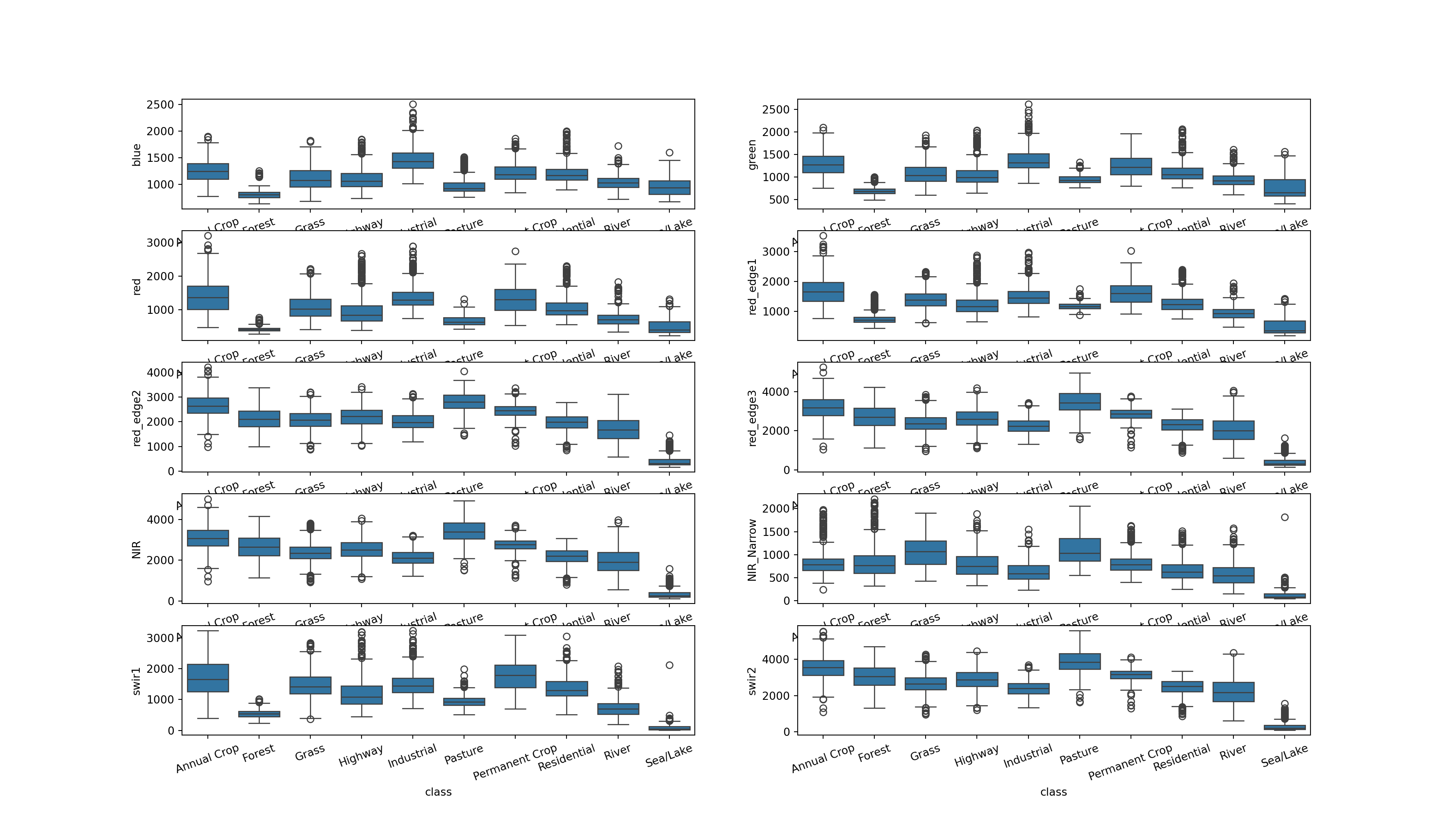
Build Fully Connected Neural Network
I am now ready to define a fully connected neural network. This is the same network that I defined in the first module focused on learning how to subclass nn.Module. Again, the __init__() constructor method defines the parameters and the components of the model. Here, I am using nn.Sequential() to define the series of layers. Remember that the input size of a layer must be equal to the output size of the prior layer. The first input size must be equal to the number of input predictor variables, in this case 10, and the final output size must be equal to the number of classes being differentiated, in this case 10. If this were a regression problem, there would only be 1 output node. If it were a binary classification, there could be 1 or 2 output nodes. The __forward__() method defines how the data will be passed through the network. The network will return the final logits for each class. Since I will be using nn.CrossEntropyLoss() as the loss metric, the model should output logits as opposed to class probabilities since this function incorporates the softmax activation into its computation.
class myFCN(nn.Module):
  def __init__(self, inSize, hiddenSizes, outSize):
    super().__init__()
    self.inSize = inSize
    self.hiddenSize = hiddenSizes
    self.outSize = outSize

    self.theNetwork = nn.Sequential(
        nn.Linear(inSize, hiddenSizes[0]),
        nn.BatchNorm1d(hiddenSizes[0]),
        nn.ReLU(inplace=True),
        nn.Linear(hiddenSizes[0], hiddenSizes[1]),
        nn.BatchNorm1d(hiddenSizes[1]),
        nn.ReLU(inplace=True),
        nn.Linear(hiddenSizes[1], outSize)
    )

  def forward(self, x):
    x = self.theNetwork(x)
    return x
I next instantiate an instance of myFCN called model with an input size of 10, 256 neurons in each of the two hidden layers, and an output size of 10. The model is moved to the defined device, in my case the GPU, using the to() method.
Lastly, I call the model to inspect it. Again, it is good to summarize or print the model and make sure no issues are observed. In this case, the sequence and the input and output sizes of each fully connected layer look correct.
model = myFCN(10, [256, 256], 10).to(device)modelmyFCN(
(theNetwork): Sequential(
(0): Linear(in_features=10, out_features=256, bias=True)
(1): BatchNorm1d(256, eps=1e-05, momentum=0.1, affine=True, track_running_stats=True)
(2): ReLU(inplace=True)
(3): Linear(in_features=256, out_features=256, bias=True)
(4): BatchNorm1d(256, eps=1e-05, momentum=0.1, affine=True, track_running_stats=True)
(5): ReLU(inplace=True)
(6): Linear(in_features=256, out_features=10, bias=True)
)
)Define Training Loop and Train the Model
I am now ready to train the model. First, I define an optimizer, in this case AdamW, which is an augmentation of mini-batch stochastic gradient descent. I also define the loss metric as cross entropy loss using nn.CrossEntropyLoss(). I reference it to the variable criterion and move it to the device.
Next, I define some additional assessment metrics using the torchmetrics package. Specifically, I will calculate overall accuracy (acc), class-aggregated F1-score (f1), and Cohen’s Kappa (kappa). Since this is a multiclass classification problem as opposed to a binary classification problem, the task parameter must be set to “multiclass”. I must also specify the number of classes being differentiated. Finally, each metric is moved to the device.
The torchmetrics package has other parameters that can be specified for assessment metrics. For example, you can set a multidimensional averaging method that defines how dimensions are handled or reduced. Here, all dimensions are flattened, which is the default. You can also choose to ignore an index in the calculation. This is sometimes used if you have a “not labeled” or “missing” class that should not be considered in the loss calculation, backpropagation, and optimization. If you want to learn more about the torchmetrics package, please consult the associated documentation: https://torchmetrics.readthedocs.io/en/stable/.
optimizer = torch.optim.AdamW(model.parameters())criterion = nn.CrossEntropyLoss().to(device)acc = tm.Accuracy(task="multiclass", num_classes=10).to(device)
f1 = tm.F1Score(task="multiclass", average="macro", num_classes=10).to(device)
kappa = tm.CohenKappa(task="multiclass", num_classes=10).to(device)Lastly, I define the number of training epochs and a folder in which to save the trained models.
epochs = 100
saveFolder = "C:/datasets/eurosat_fcnn_models/"
I am now ready to train the model using a training loop. The defined loop is more complicated than the one that I defined for the linear regression model in a prior module. Now, I will be training using mini-batches. I have also integrated in a validation set and multiple assessment metrics. Let’s step through this training loop to make sure you understand the process, components, and associated logic.
- I initialize a series of empty lists which will store the losses and assessment metrics calculated during each epoch. A total of 9 lists are created to store the epoch number (eNum), training loss (t_loss), training overall accuracy (t_acc), training F1-score (t_f1), training Kappa (t_kappa), validation loss (v_loss), validation accuracy (v_acc), validation F1-score (v_f1), and validation Kappa (v_kappa).
- The training loop will iterate over the number of epochs. This is the outer most for loop. At the beginning of each training epoch the model is placed in training mode using model.train() and a running loss is initiated with a value of 0.0;
- For the training data, it will iterate over the mini-batches as define by the DataLoader. I use enumerate() here since I need access to both the data and the associated index within the loop.
- Within the training portion of the loop, the following steps occur: (1) a mini-batch is read in and moved to the device with the predictor variables (inputs) and labels (targets) stored in separate tensors; (2) the gradients are cleared so that each iteration of the loop is an independent weight update; (3) the model is applied to predict to the predictor variables; (4) the loss is calculated using the predictions and labels; (5) the loss for the mini-batch is added to the running loss; (6) the assessment metrics are calculated using the predictions and labels; (7) backpropagation is performed; and (8) an optimization step is performed to update the weights/parameters.
- After one complete iteration over all of the training mini-batches (i.e., one training epoch), the average loss for the entire epoch is calculated by dividing the running loss by the number of epochs; the assessment metrics are accumulated across epochs; a result is printed consisting of the epoch number, the training loss, the training accuracy, the training class-aggregated F1-score, and the training Kappa. The epoch number, training loss, and accumulated assessment metrics are saved to the list objects. Since the accuracy, F1-score, and Kappa statistic are stored as tensors on the GPU, they must be detached, moved to the CPU, and converted to numpy arrays prior to being appended to the list.
- At the end of each training epoch, the validation data are predicted in a separate loop over the validation mini-batches. This occurs after setting the model in evaluation mode using model.eval() and with the condition: with torch.no_grad(). This is so that the validation data predictions and loss calculations do not impact the gradients. Again, the model should not learn from the validation data, as this would be a data leak. In such a case, the validation data would not offer an unbiased assessment of model validation. Before looping over the validation mini-batches, a running loss for the validation mini-batches is initiated with an initial value of 0.0.
- For each validation mini-batch: (1) the predictor variables and targets are read and moved to the device; (2) the model is used to predict to the predictor variables; (3) the loss is calculated using the predictions and target labels; (4) the loss for the mini-batch is added to the running loss; and (4) the assessment metrics are calculated for each mini-batch.
- Once all of the validation mini-batches have been predicted: (1) the average loss for the entire validation epoch is calculated by dividing the running loss by the number of validation epochs; (2) the assessment metrics are accumulated across the mini-batches; (3) a print statement is provided that includes the validation loss, validation accuracy, validation class-aggregated F1-score, and validation Kappa statistic; (4) the validation loss and assessment metrics are appended to the lists (Again, the assessment metrics must be moved to the CPU and converted to numpy arrays prior to being appended); and (5) the validation assessment metrics are reset.
- At the end of each epoch the resulting model weights are saved to disk and a print statement is logged to the console.
eNum = []
t_loss = []
t_acc = []
t_f1 = []
t_kappa = []
v_loss = []
v_acc = []
v_f1 = []
v_kappa = []

# Loop over epochs
for epoch in range(1, epochs+1):
    model.train()
    #Initiate running loss for epoch
    running_loss = 0.0
    # Loop over training batches
    for batch_idx, (inputs, targets) in enumerate(trainDL):
        # Get data and move to device
        inputs, targets = inputs.to(device), targets.to(device)

        # Clear gradients
        optimizer.zero_grad()
        # Predict data
        outputs = model(inputs)
        # Calculate loss
        loss = criterion(outputs, targets)

        # Calculate metrics
        accT = acc(outputs, targets)
        f1T = f1(outputs, targets)
        kappaT = kappa(outputs, targets)

        # Backpropagate
        loss.backward()

        # Update parameters
        optimizer.step()

        #Update running with batch results
        running_loss += loss.item()

    # Accumulate loss and metrics at end of training epoch
    epoch_loss = running_loss/len(trainDL)
    accT = acc.compute()
    f1T = f1.compute()
    kappaT = kappa.compute()

    # Print Losses and metrics at end of training epoch
    print(f'Epoch: {epoch}, Training Loss: {epoch_loss:.4f}, Training Accuracy: {accT:.4f}, Training F1: {f1T:.4f}, Training Kappa: {kappaT:.4f}')

    # Append results
    eNum.append(epoch)
    t_loss.append(epoch_loss)
    t_acc.append(accT.detach().cpu().numpy())
    t_f1.append(f1T.detach().cpu().numpy())
    t_kappa.append(kappaT.detach().cpu().numpy())

    # Reset metrics
    acc.reset()
    f1.reset()
    kappa.reset()

    #Set model in evaluation model
    model.eval()
    # loop over validation batches
    with torch.no_grad():
        #Initialize running validation loss
        running_loss_v = 0.0
        for batch_idx, (inputs, targets) in enumerate(valDL):
            # Get data and move to device
            inputs, targets = inputs.to(device), targets.to(device)

            # Predict data
            outputs = model(inputs)
            # Calculate validation loss
            loss_v = criterion(outputs, targets)

            #Update running with batch results
            running_loss_v += loss_v.item()

            # Calculate metrics
            accV = acc(outputs, targets)
            f1V = f1(outputs, targets)
            kappaV = kappa(outputs, targets)

    #Accumulate loss and metrics at end of validation epoch
    epoch_loss_v = running_loss_v/len(valDL)
    accV = acc.compute()
    f1V = f1.compute()
    kappaV = kappa.compute()

    # Print validation loss and metrics
    print(f'Validation Loss: {epoch_loss_v:.4f}, Validation Accuracy: {accV:.4f}, Validation F1: {f1V:.4f}, Validation Kappa: {kappaV:.4f}')

    # Append results
    v_loss.append(epoch_loss_v)
    v_acc.append(accV.detach().cpu().numpy())
    v_f1.append(f1V.detach().cpu().numpy())
    v_kappa.append(kappaV.detach().cpu().numpy())

    # Reset metrics
    acc.reset()
    f1.reset()
    kappa.reset()

    # Save model to disk
    torch.save(model.state_dict(), saveFolder + 'eurosat_model_' + str(epoch) + '.pt')
    print(f'Model saved for epoch {epoch}.')
Before moving on, here are a few notes about training loops. Remember that it is very important to clear the gradients at the beginning of each iteration over the training mini-batches. Weight updates happen at the end of each training mini-batch and should not be impacted by prior gradients. It is also important to make sure that the prediction of the validation data and the associated calculation of the validation loss not impact the weight updates. This can be accomplished by using with torch.no_grad(). When using the torchmetrics package, it is important to remember to accumulate the metrics at the end of each epoch using the compute() method. Once the accumulated metrics are computed they should be reset using the reset() method.
It is important to understand that the validation data are only being predicted at the end of each training epoch as opposed to after each processing of a training mini-batch. So, the loop will iterate over all of the training mini-batches and update the weights after each mini-batch before it predicts to the validation data.
It would be possible to only save the model if an improvement is found from the prior epoch. Or, I could only save one model to disk, which is overwritten if the current epoch offers and improvement, as opposed to saving each model. This is especially preferred when we are training over a lot of epochs or when the model has a lot of trainable parameters and the associated weight /parameter files are large. This will be demonstrated in later modules. Here, each model save is not very large.
Lastly, it will take some time to train this model. On my machine it took roughly 15 minutes. However, this will vary based on your hardware. Training this model on a CPU is possible but would greatly increase the training time. If you don’t want to run the model, the last section of this module shows how to load the saved weights from the training process. These weights have been provided in the class data folder.
Visualize Learning Process
Now that I have a trained model, let’s take a look at the results. I first combine all of the losses and assessment metrics into a single DataFrame. This requires converting each list to a pandas Series then using the concat() function from pandas to merge them into a DataFrame. I set the axis argument to 1 so that each Series will be treated as a column as opposed to a row. In other words, each row will represent the data for one training epoch.
I next call the DataFrame to view the results, save it to disk as a CSV file, then read the results back in to the workflow.
SeNum = pd.Series(eNum, name="epoch")
St_loss = pd.Series(t_loss, name="training_loss")
St_acc = pd.Series(t_acc, name="training_accuracy")
St_f1 = pd.Series(t_f1, name="training_f1")
St_kappa = pd.Series(t_kappa, name="training_kappa")
Sv_loss = pd.Series(v_loss, name="val_loss")
Sv_acc = pd.Series(v_acc, name="val_accuracy")
Sv_f1 = pd.Series(v_f1, name="val_f1")
Sv_kappa = pd.Series(t_kappa, name="val_kappa")
resultsDF = pd.concat([SeNum, St_loss, St_acc, St_f1, St_kappa, Sv_loss, Sv_acc, Sv_f1, Sv_kappa], axis=1)resultsDF.head()resultsDF.to_csv("data/models/eurosat_fcnn_results.csv")resultsDF = pd.read_csv("data/models/eurosat_fcnn_results.csv")I next use matplotlib to plot the losses and class-aggregated F-1 scores by epoch. Generally, the model seems to work well. The loss was reduced as the weights were updated at the end of each training batch. The losses for the validation data were not that different from those for the training data, suggesting that overfitting was not an issue. It might be worth training the algorithm for more epochs to see if there is any additional improvement; however, the training and validation losses do appear to have leveled off after ~50 epochs using the default learning rate.
When plotting the F1-score, we tend to see a smoother increase for the training data as opposed to the validation data. This is expected, since the training data are being used to update the weights and the validation data are not. It appears that the F1-score for the training data was still increasing when the training process ended. However, the validation F1-score has appeared to level off. This could indicate that training for a larger number of epochs could result in overfitting. In other words, the model would start to memorize the training data as opposed to learning generalizable patterns. This highlights the importance of incorporating a validation dataset into the training process.
You may have noticed that the last model, or the set of weights after 100 epochs, did not provide the highest accuracy or lowest loss for predicting to the validation data. So, you may choose to use the weights from a prior epoch as the final model. When determining which model to use as your final model, which will be applied to the testing data, used to infer to new data, and used as the final product from the training process, you can make a decision based on which weight set provided the highest class-aggregated F1-score for predicting to the validation data or some other criteria.
plt.rcParams['figure.figsize'] = [10, 10]
firstPlot = resultsDF.plot(x='epoch', y="training_loss")
resultsDF.plot(x='epoch', y="val_loss", ax=firstPlot)
plt.show()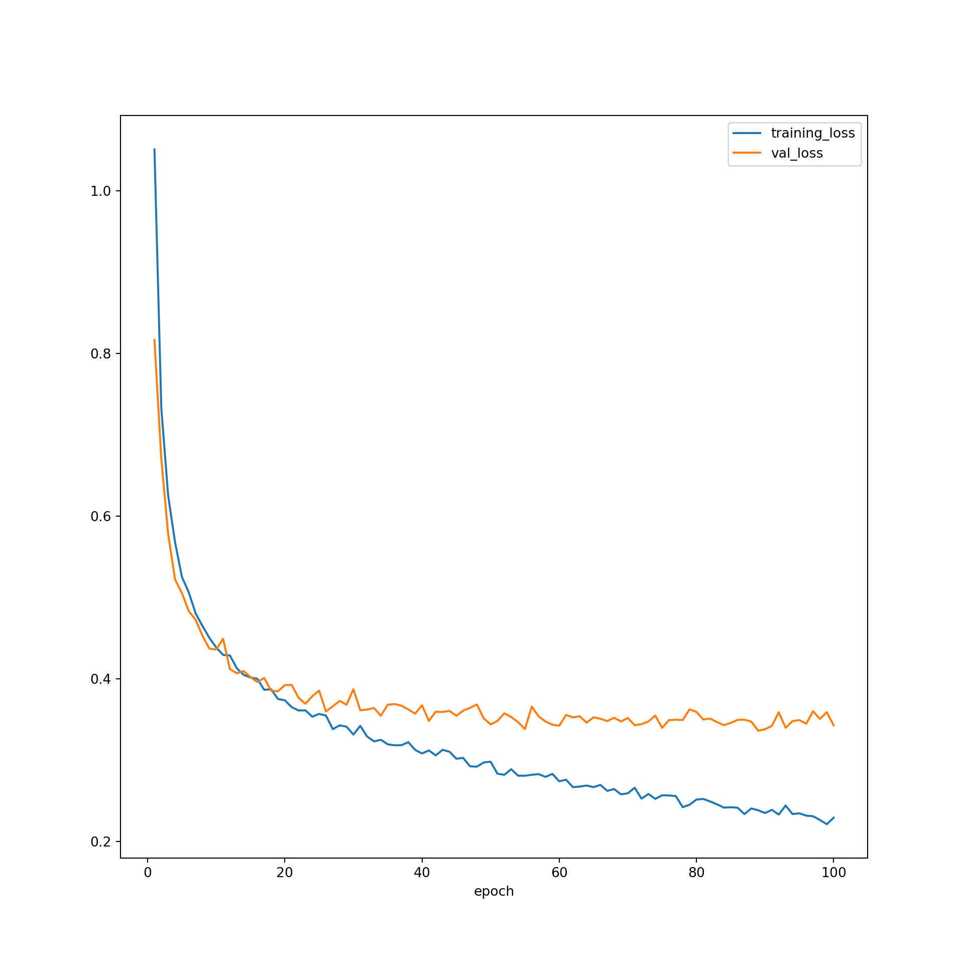
plt.rcParams['figure.figsize'] = [10, 10]
firstPlot = resultsDF.plot(x="epoch", y="training_f1")
resultsDF.plot(x='epoch', y="val_f1", ax=firstPlot)
plt.show()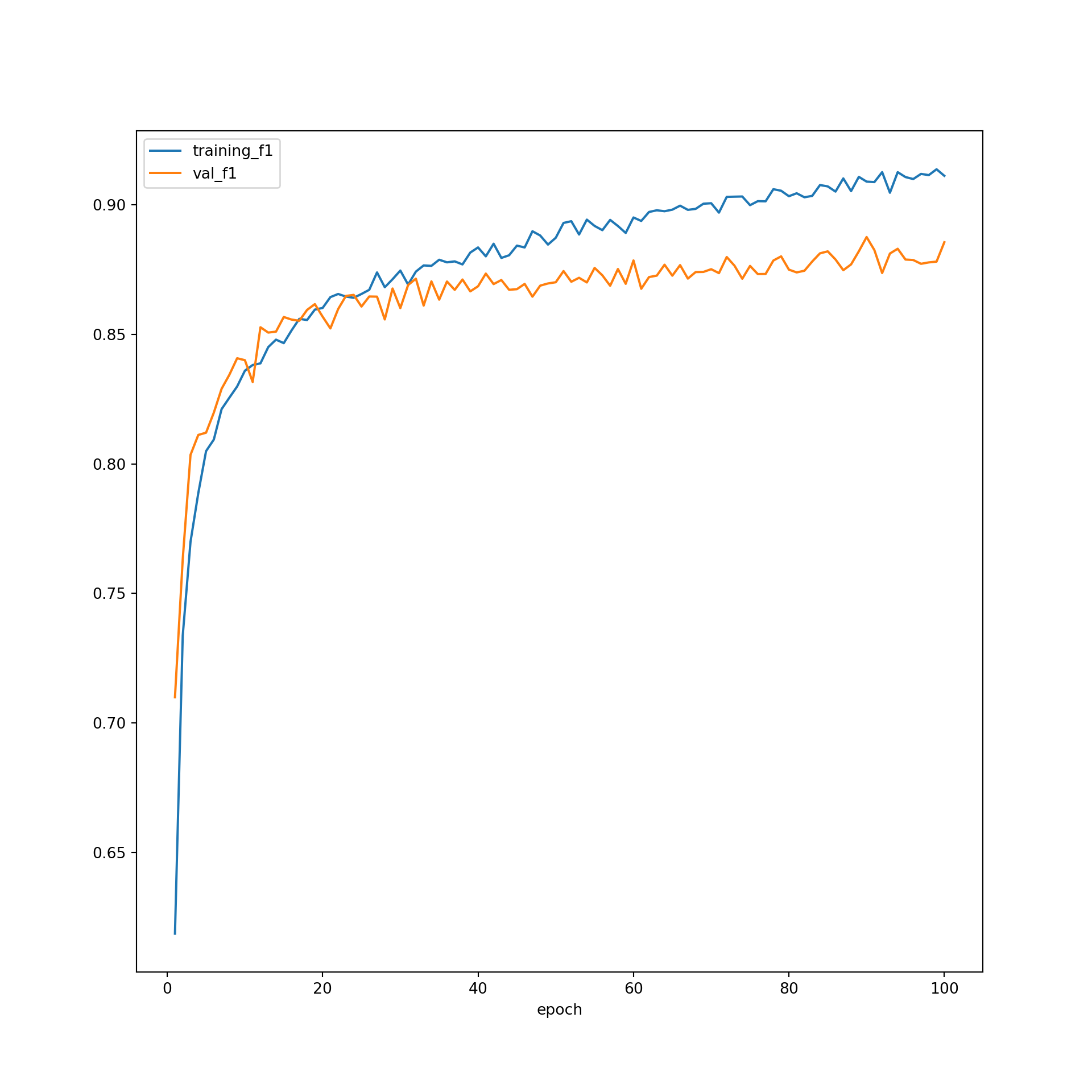
Model Validation
Let’s use a saved model to predict to the testing dataset. I first load the saved model from disk. You can load the provided model if you want to run the the code below without executing the training loop above. How this is done will be described in the next section. The code below is very similar to the validation component of the training loop except that it is not embedded inside of the training loop. In order to make sure that this inference and assessment process does not impact the gradients, I place the model in evaluation mode using the eval() method. I loop over the testing data batches and calculate the loss and assessment metrics. The assessment metrics are then accumulated using the compute() method then reset at the end of the process.
model = myFCN(10, [256, 256], 10).to(device)
saveFolder = "C:/datasets/models/"
best_weights = torch.load('data/models/eurosat_fcnn_model.pt')
model.load_state_dict(best_weights)
<All keys matched successfully>model.eval()myFCN(
(theNetwork): Sequential(
(0): Linear(in_features=10, out_features=256, bias=True)
(1): BatchNorm1d(256, eps=1e-05, momentum=0.1, affine=True, track_running_stats=True)
(2): ReLU(inplace=True)
(3): Linear(in_features=256, out_features=256, bias=True)
(4): BatchNorm1d(256, eps=1e-05, momentum=0.1, affine=True, track_running_stats=True)
(5): ReLU(inplace=True)
(6): Linear(in_features=256, out_features=10, bias=True)
)
)running_loss_v = 0.0
with torch.no_grad():
for batch_idx, (inputs, targets) in enumerate(testDL):
inputs, targets = inputs.to(device), targets.to(device)
outputs = model(inputs)
loss_v = criterion(outputs, targets)
accV = acc(outputs, targets)
f1V = f1(outputs, targets)
kappaV = kappa(outputs, targets)
running_loss_v = loss_v.item()
epoch_loss_v = running_loss_v/len(testDL)
accV = acc.compute()
f1V = f1.compute()
kappaV = kappa.compute()
acc.reset()
f1.reset()
kappa.reset()After this inference process is completed, I print the results. I obtained an overall accuracy of 88.2%, a class-aggregated, macro-averaged F1-score of 0.874, and a Kappa statistic of 0.869. Generally, this suggests fairly strong model performance. Roughly ~88% of the withheld test samples were correctly classified. I would argue that this is a pretty decent result given that I only used the band means as predictor variables and because the network was pretty simple. We will explore making predictions using the images and CNN architectures in later modules, and it will be interesting to see what improvement this may provide.
It should be noted that this is a simple model. Better performance could potentially be obtained using complex architectures and/or a more customized or refined training process.
print(accV)tensor(0.9234, device='cuda:0')print(f1V)tensor(0.9181, device='cuda:0')print(kappaV)tensor(0.9146, device='cuda:0')print(epoch_loss_v)0.006783013994043524It is possible to obtain class-level metrics as opposed to class-aggregated metrics when using torchmetrics by setting the average parameter to “none”. In the example below, I have obtained the entire confusion matrix and the F1-score, recall, and precision metrics for each class by re-instantiating the metrics, as implemented in torchmetrics, with the average parameter set to “none”. I then re-execute the evaluation loop, which includes computing the metrics and aggregating them across the data mini-batches.
cm = tm.ConfusionMatrix(task="multiclass", num_classes=10).to(device)
f1 = tm.F1Score(task="multiclass", num_classes=10, average="none").to(device)
recall = tm.Precision(task="multiclass", num_classes=10, average="none").to(device)
precision = tm.Recall(task="multiclass", num_classes=10, average="none").to(device)model.eval()myFCN(
(theNetwork): Sequential(
(0): Linear(in_features=10, out_features=256, bias=True)
(1): BatchNorm1d(256, eps=1e-05, momentum=0.1, affine=True, track_running_stats=True)
(2): ReLU(inplace=True)
(3): Linear(in_features=256, out_features=256, bias=True)
(4): BatchNorm1d(256, eps=1e-05, momentum=0.1, affine=True, track_running_stats=True)
(5): ReLU(inplace=True)
(6): Linear(in_features=256, out_features=10, bias=True)
)
)with torch.no_grad():
for batch_idx, (inputs, targets) in enumerate(testDL):
inputs, targets = inputs.to(device), targets.to(device)
outputs = model(inputs)
cmV = cm(outputs, targets)
f1V = f1(outputs, targets)
pV = precision(outputs, targets)
rV = recall(outputs, targets)
cmV =cm.compute()
f1V = f1.compute()
pV = precision.compute()
rV = recall.compute()
cm.reset()
f1.reset()
precision.reset()
recall.reset()print(cmV)tensor([[571, 0, 0, 16, 2, 2, 4, 3, 2, 0],
[ 0, 599, 0, 0, 0, 1, 0, 0, 0, 0],
[ 1, 0, 582, 11, 3, 1, 1, 1, 0, 0],
[ 32, 11, 9, 342, 21, 11, 18, 39, 17, 0],
[ 0, 0, 1, 20, 457, 0, 1, 18, 3, 0],
[ 1, 0, 2, 11, 0, 386, 0, 0, 0, 0],
[ 11, 0, 3, 11, 3, 2, 461, 6, 3, 0],
[ 0, 0, 2, 30, 17, 0, 1, 549, 1, 0],
[ 3, 5, 3, 43, 3, 7, 1, 2, 431, 2],
[ 1, 0, 0, 0, 0, 0, 0, 0, 0, 719]], device='cuda:0')print(f1V)tensor([0.9361, 0.9860, 0.9684, 0.6951, 0.9085, 0.9531, 0.9341, 0.9015, 0.9007,
0.9979], device='cuda:0')print(pV)tensor([0.9517, 0.9983, 0.9700, 0.6840, 0.9140, 0.9650, 0.9220, 0.9150, 0.8620,
0.9986], device='cuda:0')print(rV)tensor([0.9210, 0.9740, 0.9668, 0.7066, 0.9032, 0.9415, 0.9466, 0.8883, 0.9431,
0.9972], device='cuda:0')Save to and Load Models from Disk
In this last section, I will show you how to load saved weights/parameters into a model. As you saw in the training loop above, weights can be saved to disk using the torch.save() function. This specifically saves the model state dictionary, which contains the set of learned weights/parameters. In order to load these weights/parameters into a model, I need to (1) instantiate a new instance of the model with the correct architecture, (2) use torch.load() to load the weights from the file saved to disk, then (3) update the state dictionary with these weights using the load_state_dict() method for the model instance. Note that the weights/parameters will fail to load if they cannot be mapped to the correct components of the model. This will happen if the instantiated model has a different architecture than the trained model from which the weights originated.
Once the weights are loaded in, the model can be used to infer to new data. You can also load weights then continue to train the model starting from these weights as opposed to random weights. Again, if you do not have the time or hardware to train the model, you can use the provided weight/parameter file. Generally, inference is much less computationally demanding than training.
class myFCN(nn.Module):
  def __init__(self, inSize, hiddenSizes, outSize):
    super().__init__()
    self.inSize = inSize
    self.hiddenSize = hiddenSizes
    self.outSize = outSize

    self.theNetwork = nn.Sequential(
        nn.Linear(inSize, hiddenSizes[0]),
        nn.BatchNorm1d(hiddenSizes[0]),
        nn.ReLU(inplace=True),
        nn.Linear(hiddenSizes[0], hiddenSizes[1]),
        nn.BatchNorm1d(hiddenSizes[1]),
        nn.ReLU(inplace=True),
        nn.Linear(hiddenSizes[1], outSize)
    )

  def forward(self, x):
    x = self.theNetwork(x)
    return x
model = myFCN(10, [256,256], 10)model = myFCN(10, [256, 256], 10).to(device)
saveFolder = "C:/datasets/models/"
best_weights = torch.load(saveFolder+'eurosat_fcnn_model.pt')
model.load_state_dict(best_weights)Concluding Remarks
Now that you have knowledge of network architectures, optimizers, losses, assessment metrics, DataSet subclassing, DataLoaders, using training loops to update model weights, and assessing models with withheld data, you should be able to implement basic PyTorch workflows. In the following section, we will investigate some common methods used to potentially improve model performance. This will conclude the first section of the course. Next, we will start exploring convolutional neural networks that allow for the incorporation of spatial context into the learning process. Although this process is a bit different, you will find that what you have learned so far will carry over substantially.
If you are interested in exploring fully connected neural networks further, you could use the methods that we have discussed over the last series of modules to investigate specific research questions such as the following:
How does using only the visible band means compare to using all the band means in regards to model performance?
How is the model performance impacted by changing the number of hidden layers or the number of nodes in each hidden layer?
How does changing the learning rate impact the model performance? How about using a different optimizer?
How is model performance impacted by reducing the training sample size?
How does removing the batch normalization layers impact model performance?