Improving Model Performance

Improving Model Performance

Introduction

Before moving on to discuss convolutional neural networks, I wanted to take some time to discuss methods that are commonly used to attempt to improve model performance. In its current state, deep learning is science, art, and tradecraft. As a result, analysts learn with time and experience what techniques may help them achieve more accurate and generalizable models. Unfortunately, due to the complexity of these models and the methods used to train them, it is not possible to assess all possible options to potentially improve models. Instead, individuals must build intuition as to what methods might be most appropriate for their specific use case or application domain. With that said, there are some commonly used techniques that are often explored, and those are the focus of this section. Note that I am saving a discussion of some specific methods for later modules.

Methods that are often explored to potentially improve model performance include the following.

1. Collecting more or better training data. Deep learning models tend to be data hungry, partially due to the large number of parameters that must be estimated and the issue of overfitting. As a result, adding training samples is an often first suggestion to improve model performance. Unfortunately, it is not always practical or possible to collect more data. Further, the number of samples that are needed to successfully train a model without overfitting is not generally clearly defined. This is often case specific.
2. It is possible to initialize models using weights/parameters learned from other datasets. For example, large datasets, such as ImageNet and Common Objects in Context (COCO), can be used to train models. The learned weights can be used as a starting point to then apply the model to a new problem or dataset. This can be accomplished by either initializing the model using these learned weights, essentially using these weights as a starting point as opposed to using a random initialization. Alternatively, portions of the model can be frozen and only a subset of the weights can be updated. The process of using weights that were learned from another, and often much larger, dataset is called transfer learning. We will discuss transfer learning in later modules, so will not cover it in this section.
3. In order to reduce overfitting and improve model generalization, it is common to augment the input data. Using images as an example, random flips, rotations, sharpening, blurring, and/or adjustments to saturation, contrast, and/or brightness can be applied. This is termed image augmentation, and the idea is that creating more variability in the training data can result in a more varied representation and thus discourage overfitting to the training data. We will explore data augmentations in the context of convolutional neural networks for scene labeling and semantic segmentation tasks in later modules.
4. Data imbalance can have a negative impact on the learning process. Classes that make up a larger proportion of the training dataset will have a larger impact on the learning process and the calculated losses; as a result, the model will tend to focus more on these classes as opposed to less abundant classes. Practically, this can result in the model doing a poorer job at predicting the less abundant classes, overpredicting the abundance of the more prominent classes, and/or underpredicting the abundance of the less prominent classes. There are several methods to combat overfitting including using class weightings in the loss metric calculations, using loss metrics that are less impacted by class imbalance, and/or augmenting the training data so that classes are represented with more even abundance. We will discuss these methods in this section.
5. The model architecture can also be altered to potentially improve model performance. Common modifications include integrating batch normalization and/or dropouts, increasing the complexity of the network so that it can model more complex patterns in the data, and using different activation functions. We will discuss some of these methods in this section. One issue here is that increasing the complexity of the network can result in overfitting and reduced generalization, especially if the training dataset is small. Thus, increasing the size and complexity of the model architecture may not have the desired effect. A lot of convolutional neural network architectures have been specifically designed and proposed to deal with the issue of capturing complex patterns while not overfitting to the training dataset. We will discuss some of these architectures and logic behind them in later sections.
6. The optimization algorithm used can have a large impact on the modeling process, and there are many alternatives to traditional stochastic gradient descent that are derived from and build on this method. I generally use the AdamW optimizer as a default. However, people have varying opinions about the best optimizer for a specific use case. They all have pros and cons.
7. Regardless of the optimizer used, the selected learning rate can have a large impact on model performance. My go-to first attempts to potentially improve model performance are (1) to change or augment the loss function being used and/or (2) to adjust the learning rate. There are other optimizer-specific settings that can impact the learning process as well. One means to select the learning rate specifically is to make use of a learning rate finder. We will discuss learning rate finders in this section.
8. It is possible to augment the learning rate, or other parameter settings, during the learning process. In PyTorch this is generally implemented using schedulers. We will explore schedulers in this section.
9. There are other training loop modifications that may also be helpful. In this section, we will explore gradient accumulation.

Preparation

As normal, I begin with imports. I also set the device variable. Here, I am specifically making use of a GPU to potentially speed up computation.

import numpy as np
import pandas as pd
import matplotlib
from matplotlib import pyplot as plt 
import seaborn as sns
plt.rcParams['figure.figsize'] = [20, 20]

import os
import random

from sklearn.utils.class_weight import compute_class_weight

import torch
import torch.nn as nn
import torch.nn.functional as F
from torch.utils.data.dataset import Dataset
from torch.utils.data import DataLoader

import torchmetrics as tm

device = torch.device("cuda:0" if torch.cuda.is_available() else "cpu")
print(device)

cuda:0

I will use the same data and problem that we have been exploring: the differentiation of land cover types using band means derived from the EuroSatAllBands dataset. There is nothing new in the code blocks below. Here is a quick review of the data preparation process.

1. Read in the data tables of band means
2. Calculate the means and standard deviations from the training dataset
3. Define a DataSet subclass
4. Instantiate the datasets and normalize the band means
5. Instantiate the DataLoaders

folder = "C:/myFiles/work/dl/eurosat/EuroSATallBands/"
trainAgg = pd.read_csv(folder + "train_aggregated.csv")
testAgg = pd.read_csv(folder + "test_aggregated.csv")
valAgg = pd.read_csv(folder + "val_aggregated.csv")

trainAgg.head()

   Unnamed: 0       class  code  ...  NIR_Narrow        swir1        swir2
0           0  AnnualCrop     0  ...  674.346680  1461.915527  3229.570801
1           1  AnnualCrop     0  ...  758.629395  1189.456543  2714.708008
2           2  AnnualCrop     0  ...  761.717041  1621.122070  3900.247314
3           3  AnnualCrop     0  ...  638.532471  1469.149170  3986.078125
4           4  AnnualCrop     0  ...  948.018066  1656.648682  3609.164551

[5 rows x 13 columns]

trainAggMns = np.array(trainAgg.iloc[:,3:].mean(axis=0)).flatten()
print(trainAggMns)

[1116.07645724 1035.31213955  937.87729602 1184.29159721 1971.09456594
 2334.38145703 2262.04021603  724.95266414 1103.83350066 2552.01787743]

trainAggSDs = np.array(trainAgg.iloc[:,3:].std(axis=0)).flatten()
print(trainAggSDs)

[ 255.54328897  312.29876238  479.85770488  500.93361557  779.66575883
  976.84613356  970.08515215  384.49257895  670.88688372 1120.89990655]

class EuroSat(Dataset):
    
    def __init__(self, df, bndMns, bndSDs):
        super().__init__
        self.df = df
        self.bndMns = bndMns
        self.bndSDs = bndSDs
    
    def __getitem__(self, idx):
        bands = [self.df.iloc[idx, 3:]]
        label = [self.df.iloc[idx, 2]]
        bands = np.array(bands)
        bands = (bands-self.bndMns)/self.bndSDs
        label = np.array(label)
        bands = bands.astype('float32')
        bands = torch.from_numpy(bands).squeeze().float()
        label = torch.from_numpy(label).squeeze().float()
        label = label.long()
        return bands, label 
        
    def __len__(self):
        return len(self.df)

trainDS = EuroSat(trainAgg, trainAggMns, trainAggSDs)
testDS = EuroSat(testAgg, trainAggMns, trainAggSDs)
valDS = EuroSat(valAgg, trainAggMns, trainAggSDs)

trainDL = torch.utils.data.DataLoader(trainDS, batch_size=256, shuffle=True, sampler=None,
num_workers=0, pin_memory=False, drop_last=False)
testDL = torch.utils.data.DataLoader(testDS, batch_size=256, shuffle=True, sampler=None,
num_workers=0, pin_memory=False, drop_last=False)
valDL = torch.utils.data.DataLoader(valDS, batch_size=256, shuffle=True, sampler=None,
num_workers=0, pin_memory=False, drop_last=False)

Dropouts

Dropouts are a regularization method in which certain neurons are dropped out or their associated parameters are not updated within the training loop during passes over training batches. The idea is that not updating all of the weights/parameters during each weight update can result in reduced overfitting and improved generalization. How many neurons will be dropped in each weight update is controlled by the p parameter. In the example model architecture below, I am applying dropouts between each fully connected layer, which will cause a random 30% of the neurons to not be updated with each weight/parameter update. Note that I do not use dropouts after the final fully connected layer. Dropouts are implemented in PyTorch using nn.Dropout().

There is currently some debate as to whether dropouts are still necessary. With the advent and wide adoption of batch normalization, dropouts have generally been used less frequently. Analysts are using batch normalization as a means to potentially reduce overfitting and improve generalization as opposed to dropouts, and including both dropouts and batch normalization may be unnecessary. Again, analysts have varying opinions. I generally prefer to use batch normalization as opposed to dropouts. However, you may want to experiment with dropouts as a potential means to improve model performance.

class myFCNDrop(nn.Module):
  def __init__(self, inSize, hiddenSizes, outSize):
    super().__init__()
    self.inSize = inSize
    self.hiddenSize = hiddenSizes
    self.outSize = outSize

    self.theNetwork = nn.Sequential(
        nn.Linear(inSize, hiddenSizes[0]),
        nn.Dropout(p=0.3),
        nn.ReLU(inplace=True),
        nn.Linear(hiddenSizes[0], hiddenSizes[1]),
        nn.Dropout(p=.3),
        nn.ReLU(inplace=True),
        nn.Linear(hiddenSizes[1], outSize)
    )

  def forward(self, x):
    x = self.theNetwork(x)
    return x

Leaky ReLU

One known issue with the rectified linear unit (ReLU) activation function is the issue of “dying ReLU”. Remember that this activation function works by converting negative activations to 0 and maintaining all positive activation values. If all activations are negative, then they all will be converted to 0. This will result in a gradient of 0 and not allow for weight/parameter updates. To alleviate this issue, the leaky ReLU was introduced. Instead of simply converting all negative activations to 0, negative values are maintained but with a reduced magnitude by multiplying them by a slope term that is less than 1.

In PyTorch, ReLU can be replaced with leaky ReLU by simply changing nn.ReLU() to nn.LeakyReLU. You can also set the negative slope parameter, which is 0.01 by default.

I have generally found using leaky ReLU to be useful and worth considering. It is a very simple change, and it does not add trainable parameters to the model. There are also versions of ReLU that introduce trainable parameters; however, we will not discuss those here.

class myFCNLeaky(nn.Module):
  def __init__(self, inSize, hiddenSizes, outSize):
    super().__init__()
    self.inSize = inSize
    self.hiddenSize = hiddenSizes
    self.outSize = outSize

    self.theNetwork = nn.Sequential(
        nn.Linear(inSize, hiddenSizes[0]),
        nn.BatchNorm1d(hiddenSizes[0]),
        nn.LeakyReLU(negative_slope=0.1, inplace=True),
        nn.Linear(hiddenSizes[0], hiddenSizes[1]),
        nn.BatchNorm1d(hiddenSizes[1]),
        nn.LeakyReLU(negative_slope=0.1, inplace=True),
        nn.Linear(hiddenSizes[1], outSize)
    )

  def forward(self, x):
    x = self.theNetwork(x)
    return x

Class Weighting

One means to potentially reduce the impact of class imbalance in the dataset is to apply weights to each class when performing the loss calculations. Specifically, less abundant classes should have a higher weight in the loss calculation in comparison to more abundant classes. To accomplish this, it is common to calculate weights as the inverse of their relative abundance in the dataset.

Fortunately, scikit-learn provides the compute_class_weight() function for accomplishing this. This requires to first extract the class labels into a numpy array. Setting the class_weight parameter to ‘balanced’ will yield weights that equalize the impact of each class on the weight updates. Once the weights are defined, they can be written to a torch tensor and moved to the device.

Some loss metrics allow for the incorporation of class weights. Here, I have provided an example of defining a cross entropy loss with class weights using the weight parameter in the nn.CrossEntropyLoss() implementation. To see if weights can be and how they are integrated using other loss functions, please consult the associated documentation.

It is also possible to incorporate class weights into some assessment metric calculations. Although this won’t inform the weight updates, it can be useful for selecting a model or determining whether the model is improving.

npLbls = np.array(trainAgg.iloc[:,3])

npLbls

array([1301.21630859, 1042.02490234, 1411.48461914, ...,  963.27075195,
       1153.65087891, 1105.24951172])

weights = compute_class_weight(class_weight='balanced', classes=np.unique(npLbls), y=npLbls)
weightsT = torch.tensor(weights,dtype=torch.float).to(device)

weightsT

tensor([1.0025, 1.0025, 1.0025,  ..., 1.0025, 1.0025, 1.0025], device='cuda:0')

criterion = nn.CrossEntropyLoss(weight=weightsT).to(device)

Alternative Loss Metric

Another option is to use a loss metric that is less impacted by class imbalance, such as the DICE or Tversky loss. Further, the focal Tversky loss is generally more robust to data imbalance than cross entropy loss while also allowing for defining the relative impacts of false positive and false negative errors and allowing for adjusting the impact of difficult to classify training samples. Another option is to combine loss functions to create a combination loss, such as using cross entropy loss + DICE or cross entropy loss + Tversky loss.

Generally, I have found using an alternative loss metric to be worth considering and beneficial, especially when the data are imbalanced. I generally have seen notable improvements when using DICE as opposed to cross entropy or DICE + cross entropy as opposed to just cross entropy. The Tverksy loss is useful when you want to have more control over the relative impact of false positives and false negatives.

Below, I have provided an example implementation of focal Tversky loss, which was already discussed in the Losses and Assessment Metrics module. Custom losses can be defined by subclassing nn.Module.

class FocalTverskyLoss(nn.Module):
    def __init__(self):
        super().__init__()

    def forward(self, inputs, targets, smooth=1, alpha=.5, beta=.5, gamma=1, fromProbs=False):
    
        if fromProbs == False:
          inputs = F.sigmoid(inputs)       
        
        inputs = torch.round(inputs)   
      
        TP = (inputs * targets).sum()    
        FP = ((1-targets) * inputs).sum()
        FN = (targets * (1-inputs)).sum()
       
        Tversky = (TP + smooth) / (TP + alpha*FP + beta*FN + smooth)  
        FocalTversky = (1 - Tversky)**gamma
        
        return FocalTversky

Class Balancing Dataset

Instead of augmenting the loss function to deal with class imbalance, you may choose to augment the data. One means to do this is to incorporate a sampler into the DataLoader, which is used to select which samples are provided in the training loop. Specifically, classes that are less abundant will be sampled more often than those that are less abundant.

To accomplish this, I first create a new column in the training DataFrame called “weight”. This is initially filled with the class numeric codes. I then use the pandas replace() method to replace the class codes with their desired weights, as defined using the compute_class_weight() function from scikit-learn. The weights are then converted to a tensor and moved to the device. The sampler is then defined using the WeightedRandomSampler() function from PyTorch. Lastly, I redefine the DataLoader for the training set and specify the sampler. Note that you cannot use shuffling along with a sampler.

This method can be especially useful for scene labeling tasks. However, it is more difficult to apply when the goal is pixel-level, or semantic, segmentation. This is because the sampling unit is now the pixel as opposed to the entire image chip. In these cases, I have found it to be necessary to consider a more manual augmentation of the training data. For example, you may choose to not use any or only a subset of image chips that only include pixels mapped to the background class. We will discuss this in more detail in the modules associated with semantic segmentation.

from torch.utils.data import WeightedRandomSampler

trainAgg['weight'] = trainAgg['code']

wweights= compute_class_weight(class_weight='balanced', classes=np.unique(npLbls), y=npLbls)

trainaAgg = trainAgg.replace({'weight': {0: weights[0], 
                             1: weights[1], 
                             2: weights[2],
                             3: weights[3], 
                             4: weights[4], 
                             5: weights[5],
                             6: weights[6], 
                             7: weights[7], 
                             8: weights[8], 
                             9: weights[9]}})

weightsT =torch.tensor(trainAgg["weight"], dtype=torch.float).to(device)

trainAgg.drop(['weight'], axis=1, inplace=True)

sampler = WeightedRandomSampler(
        weightsT, num_samples=len(trainAgg), replacement=True
    )

trainDL = torch.utils.data.DataLoader(trainDS, batch_size=256, shuffle=False, sampler=sampler,
num_workers=0, pin_memory=False, drop_last=False)

Learning Rate Finder

Tools have been developed to help you select an appropriate learning rate or range of learning rates. Details of how this is conducted are described in the following paper by Leslie Smith:

Smith, L.N., 2017, March. Cyclical learning rates for training neural networks. In 2017 IEEE winter conference on applications of computer vision (WACV) (pp. 464-472). IEEE.

Unfortunately, this method is not natively available in PyTorch. Instead, I will make use of the implementation provided here: https://github.com/davidtvs/pytorch-lr-finder. You will need to install this package to execute the example code.

In the provided example, I am testing learning rates between 0.0001 and 1 for up to 100 iterations. The result is a graph that depicts the loss at different learning rates. The best learning rate is defined as the one with the steepest slope.

To learn more about how this process works, please consult the paper referenced above.

#!pip install torch-lr-finder

from torch_lr_finder import LRFinder

class myFCNLeaky(nn.Module):
  def __init__(self, inSize, hiddenSizes, outSize):
    super().__init__()
    self.inSize = inSize
    self.hiddenSize = hiddenSizes
    self.outSize = outSize

    self.theNetwork = nn.Sequential(
        nn.Linear(inSize, hiddenSizes[0]),
        nn.BatchNorm1d(hiddenSizes[0]),
        nn.LeakyReLU(negative_slope=0.1, inplace=True),
        nn.Linear(hiddenSizes[0], hiddenSizes[1]),
        nn.BatchNorm1d(hiddenSizes[1]),
        nn.LeakyReLU(negative_slope=0.1, inplace=True),
        nn.Linear(hiddenSizes[1], outSize)
    )

  def forward(self, x):
    x = self.theNetwork(x)
    return x

model = myFCNLeaky(10, [256, 256], 10).to(device)

criterion = nn.CrossEntropyLoss()
optimizer = torch.optim.AdamW(model.parameters())
lr_finder = LRFinder(model, optimizer, criterion, device="cuda")
lr_finder.range_test(trainDL, val_loader=valDL, start_lr=0.0001, end_lr=1, num_iter=100, step_mode="linear")

Stopping early, the loss has diverged
Learning rate search finished. See the graph with {finder_name}.plot()


  0%|          | 0/100 [00:00<?, ?it/s]
  1%|1         | 1/100 [00:01<02:28,  1.50s/it]
  2%|2         | 2/100 [00:02<02:02,  1.25s/it]
  3%|3         | 3/100 [00:03<01:52,  1.16s/it]
  4%|4         | 4/100 [00:04<01:47,  1.12s/it]
  5%|5         | 5/100 [00:05<01:44,  1.10s/it]
  6%|6         | 6/100 [00:06<01:42,  1.09s/it]
  7%|7         | 7/100 [00:07<01:40,  1.08s/it]
  8%|8         | 8/100 [00:08<01:36,  1.05s/it]
  9%|9         | 9/100 [00:09<01:33,  1.03s/it]
 10%|#         | 10/100 [00:10<01:32,  1.03s/it]
 11%|#1        | 11/100 [00:11<01:30,  1.02s/it]
 12%|#2        | 12/100 [00:12<01:31,  1.04s/it]
 13%|#3        | 13/100 [00:14<01:38,  1.14s/it]
 14%|#4        | 14/100 [00:15<01:42,  1.20s/it]
 15%|#5        | 15/100 [00:16<01:42,  1.21s/it]
 16%|#6        | 16/100 [00:17<01:36,  1.15s/it]
 17%|#7        | 17/100 [00:18<01:31,  1.10s/it]
 18%|#8        | 18/100 [00:19<01:27,  1.07s/it]
 19%|#9        | 19/100 [00:20<01:24,  1.04s/it]
 20%|##        | 20/100 [00:21<01:22,  1.03s/it]
 21%|##1       | 21/100 [00:22<01:20,  1.02s/it]
 22%|##2       | 22/100 [00:23<01:19,  1.02s/it]
 23%|##3       | 23/100 [00:24<01:17,  1.01s/it]
 24%|##4       | 24/100 [00:25<01:16,  1.00s/it]
 25%|##5       | 25/100 [00:26<01:14,  1.00it/s]
 26%|##6       | 26/100 [00:27<01:13,  1.01it/s]
 27%|##7       | 27/100 [00:28<01:12,  1.01it/s]
 28%|##8       | 28/100 [00:29<01:10,  1.01it/s]
 29%|##9       | 29/100 [00:30<01:09,  1.02it/s]
 30%|###       | 30/100 [00:31<01:08,  1.02it/s]
 31%|###1      | 31/100 [00:32<01:07,  1.02it/s]
 32%|###2      | 32/100 [00:33<01:06,  1.02it/s]
 33%|###3      | 33/100 [00:34<01:06,  1.01it/s]
 34%|###4      | 34/100 [00:35<01:04,  1.02it/s]
 35%|###5      | 35/100 [00:36<01:04,  1.01it/s]
 36%|###6      | 36/100 [00:37<01:03,  1.02it/s]
 37%|###7      | 37/100 [00:38<01:02,  1.01it/s]
 38%|###8      | 38/100 [00:39<01:00,  1.02it/s]
 39%|###9      | 39/100 [00:40<01:00,  1.02it/s]
 40%|####      | 40/100 [00:41<00:59,  1.01it/s]
 41%|####1     | 41/100 [00:42<00:58,  1.01it/s]
 42%|####2     | 42/100 [00:43<00:57,  1.01it/s]
 43%|####3     | 43/100 [00:44<00:56,  1.01it/s]
 44%|####4     | 44/100 [00:45<00:55,  1.01it/s]
 45%|####5     | 45/100 [00:46<00:54,  1.01it/s]
 46%|####6     | 46/100 [00:47<00:53,  1.02it/s]
 47%|####6     | 47/100 [00:48<00:52,  1.01it/s]
 48%|####8     | 48/100 [00:49<00:51,  1.01it/s]
 49%|####9     | 49/100 [00:50<00:50,  1.01it/s]
 50%|#####     | 50/100 [00:51<00:49,  1.02it/s]
 51%|#####1    | 51/100 [00:52<00:48,  1.01it/s]
 52%|#####2    | 52/100 [00:53<00:47,  1.00it/s]
 53%|#####3    | 53/100 [00:54<00:46,  1.01it/s]
 54%|#####4    | 54/100 [00:55<00:45,  1.01it/s]
 55%|#####5    | 55/100 [00:56<00:44,  1.01it/s]
 56%|#####6    | 56/100 [00:57<00:43,  1.01it/s]
 57%|#####6    | 57/100 [00:58<00:42,  1.01it/s]
 58%|#####8    | 58/100 [00:59<00:41,  1.02it/s]
 59%|#####8    | 59/100 [01:00<00:40,  1.02it/s]
 60%|######    | 60/100 [01:01<00:39,  1.02it/s]
 61%|######1   | 61/100 [01:02<00:38,  1.02it/s]
 62%|######2   | 62/100 [01:03<00:37,  1.02it/s]
 63%|######3   | 63/100 [01:04<00:36,  1.02it/s]
 64%|######4   | 64/100 [01:05<00:35,  1.02it/s]
 65%|######5   | 65/100 [01:06<00:34,  1.02it/s]
 66%|######6   | 66/100 [01:07<00:33,  1.02it/s]
 67%|######7   | 67/100 [01:08<00:32,  1.02it/s]
 68%|######8   | 68/100 [01:09<00:31,  1.01it/s]
 69%|######9   | 69/100 [01:10<00:30,  1.01it/s]
 70%|#######   | 70/100 [01:11<00:29,  1.01it/s]
 71%|#######1  | 71/100 [01:12<00:28,  1.02it/s]
 72%|#######2  | 72/100 [01:13<00:27,  1.02it/s]
 72%|#######2  | 72/100 [01:14<00:28,  1.03s/it]

lr_finder.plot(log_lr=False)

LR suggestion: steepest gradient
Suggested LR: 4.14E-01
(<AxesSubplot: >, 0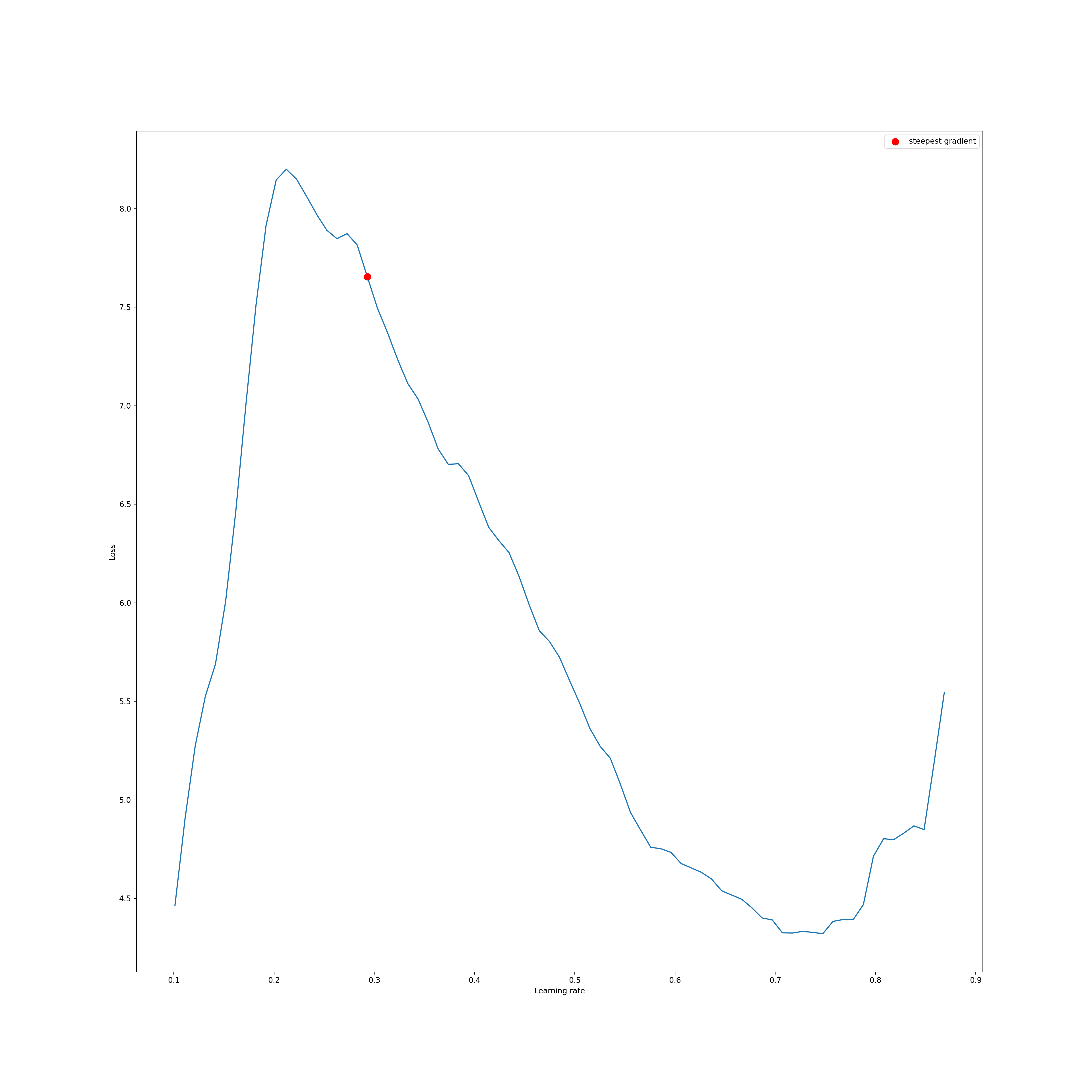.4142)

lr_finder.reset()

Learning Rate Scheduling

Another technique that has proved to be useful is augmenting the learning rate throughout the training process. There are lots of different ways to do this. One of the simplest is to use a larger learning rate early in the training then reduce the learning rate after a defined number of epochs. The idea here is that the model can be more coarsely trained initially then fine-tuned with a lower learning rate during later epochs.

One method that has been shown to be especially effective is to implement a cyclic learning rate in which the learning rate cyclically oscillates throughout the iterations over the batches and training epochs. This method was proposed by Leslie Smith in the same paper referenced above. This method has been implemented in PyTorch as a scheduler. Schedulers allow for modifying the training loop in some way by calling a step. Note that a variety of schedulers are available for different use cases. If you are interested in learning more about schedulers, please consult the PyTorch documentation.

To implement a cyclic learning rate in PyTorch, you can use the CycleLR() function. This allows for specifying the instance of the optimizer being used, a maximum learning rate, a step size when increasing the learning rate, a step size when decreasing the learning rate, and several other parameters. To actually augment the learning rate using this scheduler, you must call scheduler.step() in the training loop. Since this needs to happen at the end of batches, this should be done within the batch for loop for the training batches. In the example below, I have called it after optimizer.step(). So, this is actually pretty easy to implement. It only requires (1) defining and instantiating an instance of the scheduler and (2) performing a step within each training batch iteration in the training loop.

There are many other methods for augmenting learning rates. I recommend this post on Kaggle that demonstrates a variety of learning rate schedulers using PyTorch: https://www.kaggle.com/code/isbhargav/guide-to-pytorch-learning-rate-scheduling.

optimizer = torch.optim.SGD(model.parameters(), lr=0.1, momentum=0.9)

scheduler = torch.optim.lr_scheduler.CyclicLR(optimizer, base_lr=0.0001, max_lr=0.5, step_size_up=len(trainDL)/2, step_size_down=len(trainDL)/2)

criterion = nn.CrossEntropyLoss().to(device)

#Define assessment metrics
acc = tm.Accuracy(task="multiclass", num_classes=10).to(device)
f1 = tm.F1Score(task="multiclass", num_classes=10).to(device)
kappa = tm.CohenKappa(task="multiclass", num_classes=10).to(device)

epochs = 50

saveFolder = "C:/myFiles/work/dl/eurosat_fcnn_models/"

eNum = []
t_loss = []
t_acc = []
t_f1 = []
t_kappa = []
v_loss = []
v_acc = []
v_f1 = []
v_kappa = []

#Loop over epochs
for epoch in range(1, epochs+1):
    #Loop over batches
    for batch_idx, (inputs, targets) in enumerate(trainDL):
        #Get data and move to device
        inputs, targets = inputs.to(device), targets.to(device)

        #Clear gradients
        optimizer.zero_grad()
        #Predict data
        outputs = model(inputs)
        #Calculate loss
        loss = criterion(outputs, targets)

        #Calculate metrics
        accT = acc(outputs, targets)
        f1T = f1(outputs, targets)
        kappaT = kappa(outputs, targets)
        
        #Backpropagate
        loss.backward()

        # update parameters
        optimizer.step()
        scheduler.step()

    #Accumulate metrics at end of epoch
    accT = acc.compute()
    f1T = f1.compute()
    kappaT = kappa.compute()

    # Print Losses and metrics at end of each Epoch   
    print(f'Epoch: {epoch}, Training Loss: {loss.item():.4f}, Training Accuracy: {accT:.4f}, Training F1: {f1T:.4f}, Training Kappa: {kappaT:.4f}')

     #Append results
    eNum.append(epoch)
    t_loss.append(loss.item())
    t_acc.append(accT.detach().cpu().numpy())
    t_f1.append(f1T.detach().cpu().numpy())
    t_kappa.append(kappaT.detach().cpu().numpy())

    #Reset metrics
    acc.reset()
    f1.reset()
    kappa.reset()

    #loop over validation batches
    with torch.no_grad():
        for batch_idx, (inputs, targets) in enumerate(valDL):
            #Get data and move to device
            inputs, targets = inputs.to(device), targets.to(device)

            #Predict data
            outputs = model(inputs)
            #Calculate validation loss
            loss_v = criterion(outputs, targets)

            #Calculate metrics
            accV = acc(outputs, targets)
            f1V = f1(outputs, targets)
            kappaV = kappa(outputs, targets)
            
    #Accumulate metrics at end of epoch
    accV = acc.compute()
    f1V = f1.compute()
    kappaV = kappa.compute()

    #Print validation loss and metrics
    print(f'Validation Loss: {loss_v.item():.4f}, Validation Accuracy: {accV:.4f}, Validation F1: {f1V:.4f}, Validation Kappa: {kappaV:.4f}')

    #Append results
    v_loss.append(loss_v.item())
    v_acc.append(accV.detach().cpu().numpy())
    v_f1.append(f1V.detach().cpu().numpy())
    v_kappa.append(kappaV.detach().cpu().numpy())

    #Reset metrics
    acc.reset()
    f1.reset()
    kappa.reset()

    torch.save(model.state_dict(), saveFolder + 'eurosat_model_' + str(epoch) + '.pt')
    print(f'Model saved for epoch {epoch}.')

Gradient Accumulation

Small batch sizes can result in noisy or suboptimal weight updates. However, it is not always possible to use a large batch size. For example, if you are using large image chips, a complex architecture, and/or have limited GPU VRAM, you may not be able to use a large batch size. To get around this issue, you can implement gradient accumulation. The idea here is that the weights are not updated after each training batch. Instead, the gradients are allowed to accumulate over a given number of batches prior to performing the optimization.

In the example below, I am allowing the gradients to accumulate for 4 batches before applying the optimization or weight updates. This involves (1) defining a variable, in this case accum_iter, that specifies over how many batches to accumulate the losses over, (2) dividing the loss by this variable for normalization, (3) defining a condition with an if statement so that gradients will only be updated after every 4 batches or for the final training batch, and (5) only applying the optimizer and clearing the gradients if one of these conditions are met. In my example below, this condition is applied inside of the for loop that iterates over the batches and after the loss has been calculated and the backpropagation has been performed. Also, I am not clearing the gradients at the beginning of each training batch. Instead, this occurs within the conditions since accumulating the gradients cannot occur if they are cleared. So, the gradients are only cleared after an optimization step has been performed.

In this specific example, gradient accumulation is not necessary since the batch size is large. This is just an example.

eNum = []
t_loss = []
t_acc = []
t_f1 = []
t_kappa = []
v_loss = []
v_acc = []
v_f1 = []
v_kappa = []

accum_iter = 4

# Loop over epochs
for epoch in range(1, epochs+1):
    # Loop over training batches
    for batch_idx, (inputs, targets) in enumerate(trainDL):
        # Get data and move to device
        inputs, targets = inputs.to(device), targets.to(device)

        # Clear gradients
        optimizer.zero_grad()
        # Predict data
        outputs = model(inputs)
        # Calculate loss
        loss = criterion(outputs, targets)/accum_iter

        # Calculate metrics
        accT = acc(outputs, targets)
        f1T = f1(outputs, targets)
        kappaT = kappa(outputs, targets)
        
        # Backpropagate
        loss.backward()

        # Implement gradient accumulation
        if ((batch_idx + 1) % accum_iter == 0) or (batch_idx + 1 == len(trainDL)):
            optimizer.step()
            optimizer.zero_grad()

    # Accumulate metrics at end of epoch
    accT = acc.compute()
    f1T = f1.compute()
    kappaT = kappa.compute()

    # Print Losses and metrics at end of each training epoch   
    print(f'Epoch: {epoch}, Training Loss: {loss.item():.4f}, Training Accuracy: {accT:.4f}, Training F1: {f1T:.4f}, Training Kappa: {kappaT:.4f}')

    # Append results
    eNum.append(epoch)
    t_loss.append(loss.item())
    t_acc.append(accT.detach().cpu().numpy())
    t_f1.append(f1T.detach().cpu().numpy())
    t_kappa.append(kappaT.detach().cpu().numpy())

    # Reset metrics
    acc.reset()
    f1.reset()
    kappa.reset()

    # loop over validation batches
    with torch.no_grad():
        for batch_idx, (inputs, targets) in enumerate(valDL):
            # Get data and move to device
            inputs, targets = inputs.to(device), targets.to(device)

            # Predict data
            outputs = model(inputs)
            # Calculate validation loss
            loss_v = criterion(outputs, targets)

            # Calculate metrics
            accV = acc(outputs, targets)
            f1V = f1(outputs, targets)
            kappaV = kappa(outputs, targets)
            
    # Accumulate metrics at end of validation epoch
    accV = acc.compute()
    f1V = f1.compute()
    kappaV = kappa.compute()

    # Print validation loss and metrics
    print(f'Validation Loss: {loss_v.item():.4f}, Validation Accuracy: {accV:.4f}, Validation F1: {f1V:.4f}, Validation Kappa: {kappaV:.4f}')

    # Append results
    v_loss.append(loss_v.item())
    v_acc.append(accV.detach().cpu().numpy())
    v_f1.append(f1V.detach().cpu().numpy())
    v_kappa.append(kappaV.detach().cpu().numpy())

    # Reset metrics
    acc.reset()
    f1.reset()
    kappa.reset()

    #Save model
    torch.save(model.state_dict(), saveFolder + 'eurosat_model_' + str(epoch) + '.pt')
    print(f'Model saved for epoch {epoch}.')

Using Multiple GPUs

Training on multiple GPUs is an effective means to speed up the training process. Also, it can allow for larger batch sizes. So, if you are fortunate enough to have access to a computer with multiple CUDA-enabled GPUs or a GPU cluster, I highly recommend augmenting your code to make use of this hardware. The code below shows how to get the count of available GPUs.

devCnt = torch.cuda.device_count()

There are a few methods that can be used to train your model over multiple GPUs. I tend to use nn.DataParallel(). This allows for partitioning the training batches into multiple smaller batches that are then processed on separate GPUs in parallel.

Implementing this method is very easy. You simply need to wrap your model in this function, as demonstrated below, then move it to the device. The training loop can then be implemented as normal.

model = nn.DataParallel(model)

model.to(DEVICE)

Enhancing Reproducibility

Lastly, you may want to be able to obtain the same results when running the training process multiple times. Obtaining reproducibility is complex with PyTorch, especially when using GPU-based computation. The following paper provides some guidance on obtaining reproducibility within PyTorch:

Alahmari, S.S., Goldgof, D.B., Mouton, P.R. and Hall, L.O., 2020. Challenges for the repeatability of deep learning models. IEEE Access, 8, pp.211860-211868.

The code below demonstrates creating a function that can set multiple random seeds and other settings that should allow for reproducible results with PyTorch.

def set_seed2(seed=2019):
    random.seed(seed)
    np.random.seed(seed)
    torch.manual_seed(seed)
    torch.random.manual_seed(seed)
    torch.cuda.manual_seed(seed)
    torch.backends.cudnn.deterministic=True
    torch.backends.cudnn.benchmark=False

Concluding Remarks

The goal of this module was to introduce some common methods that can be used to potentially improve the performance of the final model and/or to combat some common issues, such as class imbalance. If you are struggling with your training process, it might be worth investigating these techniques. It is also a good idea to explore the internet, blogs, and help sites for other suggestions that might be appropriate for your specific use case. Also, deep learning techniques are still developing, so new methods may be proposed that are not presented here. With that said, I have found the methods that I discussed here to be especially useful.