Data Summarization and Statistical Tests
Summary Statistics and Statistical Tests
Objectives
- Obtain summary statistics using base R, psych, and dplyr
- Obtain summary statistics to compare groups
- Explore variable correlation
- Statistically compare the central tendency of two groups using the T-Test and Mann-Whitney U Test
- Compare multiple groups using ANOVA and the Kruskal-Wallis Test
Summary Statistics
There are many packages available in R that provide functions to summarize data. Here, I will primarily demonstrate dplyr, which we explored in the data manipulation module, and psych. I tend to use dplyr for data manipulation and summarization tasks. However, pysch is also very useful as it allows you to obtain a variety of summary statistics quickly.
First, you will need to read in the required packages. If you haven’t installed them, you will need to do so. Also, you will need to load in some example data. We will work with the high_plains_data.csv file. The elevation (“elev”), temperature (“temp”), and precipitation (“precip2”) data were extracted from digital map data provided by the PRISM Climate Group at Oregon State University. The elevation data are provided in meters, the temperature data represent 30-year annual normal mean temperature in Celsius, and the precipitation data represent 30-year annual normal precipitation in millimeters. The original digital map data have a resolution of 4-by-4 kilometers and can be obtained here. I also summarized percent forest (“per_for”) from the 2011 National Land Cover Database (NLCD). NLCD data can be obtained from the Multi-Resolution Land Characteristics Consortium (MRLC). The link at the bottom of the page provides the example data and R Markdown file used to generate this module.
library(dplyr)
library(psych)
library(car)
library(asbio)
hp_data <- read.csv("D:/mydata/summary_stats/high_plains_data.csv", sep=",", header=TRUE, stringsAsFactors=TRUE)Global Summary Statistics using dplyr and psych
I do not need all of the columns to work through the examples. So, I am using dplyr to select out only the required variables into a new data frame. Once the required columns have been extracted, I use the summary() function from base R to obtain summary information for each column. The minimum, 1st quartile, median, mean, 3rd quartile, and maximum values are returned for continuous variables. For factors, the factor levels and associated counts are returned.
Calling levels() on a factor column will print the list of factor levels. This data set contains county-level data across eight states.
Generally, I find that it is a good idea to use summary() to inspect data prior to performing any analyses.
hp_data2 <- as.data.frame(hp_data %>% select(NAME_1, STATE_NAME, TOTPOP10, POPDENS10, per_for, temp, elev, precip2))summary(hp_data2)
NAME_1 STATE_NAME TOTPOP10 POPDENS10
Lincoln County : 6 Kansas :105 Min. : 460 Min. : 0.30
Sheridan County: 5 Nebraska : 93 1st Qu.: 3307 1st Qu.: 2.70
Custer County : 4 South Dakota: 66 Median : 7310 Median : 6.40
Douglas County : 4 Colorado : 64 Mean : 31723 Mean : 48.62
Garfield County: 4 Montana : 56 3rd Qu.: 19687 3rd Qu.: 17.60
Grant County : 4 North Dakota: 53 Max. :1029655 Max. :3922.60
(Other) :462 (Other) : 52
per_for temp elev precip2
Min. : 0.00119 Min. : 0.3863 Min. : 251.7 Min. : 2.302
1st Qu.: 0.17940 1st Qu.: 6.1287 1st Qu.: 478.8 1st Qu.: 4.413
Median : 1.21404 Median : 8.7381 Median : 755.0 Median : 5.398
Mean : 6.11726 Mean : 8.5053 Mean :1026.4 Mean : 5.782
3rd Qu.: 6.31987 3rd Qu.:10.8541 3rd Qu.:1413.6 3rd Qu.: 6.831
Max. :44.73928 Max. :14.3880 Max. :3475.8 Max. :11.449
levels(hp_data2$STATE_NAME)
[1] "Colorado" "Kansas" "Montana" "Nebraska" "North Dakota"
[6] "South Dakota" "Utah" "Wyoming" The base R head() and tail() functions can be used to print the first five or last five rows of data, respectively. If you would like to print a different number of rows, you can use the optional n argument. Similar to summary(), these functions are useful for inspecting data prior to an analysis.
head(hp_data2)
             NAME_1 STATE_NAME TOTPOP10 POPDENS10      per_for      temp
1   Hinsdale County   Colorado      843       0.8 34.962703710  1.410638
2      Kiowa County   Colorado     1398       0.8  0.002119576 11.159492
3 Kit Carson County   Colorado     8270       3.8  0.021467393 10.179698
4 Las Animas County   Colorado    15507       3.2 11.687192860 10.439925
5    Lincoln County   Colorado     5467       2.1  0.043238069  9.573578
6      Logan County   Colorado    22709      12.4  0.124508994  9.749204
      elev  precip2
1 3334.739 8.002461
2 1269.637 3.842018
3 1348.005 4.354140
4 1834.354 4.247577
5 1564.500 3.762286
6 1278.252 4.252787
tail(hp_data2)
               NAME_1 STATE_NAME TOTPOP10 POPDENS10   per_for     temp     elev
484    Natrona County    Wyoming    75450      14.1 1.6269573 6.736350 1851.832
485   Niobrara County    Wyoming     2484       0.9 1.1470432 8.011750 1382.148
486     Platte County    Wyoming     8667       4.2 2.3411135 8.072507 1573.332
487 Sweetwater County    Wyoming    43806       4.2 0.1793681 5.412980 2092.429
488   Washakie County    Wyoming     8533       3.8 2.7601385 6.963218 1595.407
489     Weston County    Wyoming     7208       3.0 4.6158960 7.501733 1361.416
     precip2
484 3.233924
485 3.835656
486 3.847026
487 2.323045
488 3.260599
489 3.751864
The describe() function from the psych package can be used to obtain a variety of summary statistics for all or individual columns of data. By default it will return the mean, standard deviation, median, trimmed mean, median absolute deviation, minimum, maximum, range, skewness, kurtosis, and standard error for continuous data.
describe(hp_data2)
            vars   n     mean       sd  median  trimmed     mad    min
NAME_1*        1 489   197.06   113.04  199.00   196.78  145.29   1.00
STATE_NAME*    2 489     3.81     2.01    4.00     3.70    2.97   1.00
TOTPOP10       3 489 31722.60 92877.01 7310.00 11504.06 7227.67 460.00
POPDENS10      4 489    48.61   239.36    6.40    10.64    6.82   0.30
per_for        5 489     6.12    10.04    1.21     3.73    1.73   0.00
temp           6 489     8.51     3.09    8.74     8.55    3.55   0.39
elev           7 489  1026.36   717.62  754.99   918.55  496.27 251.72
precip2        8 489     5.78     1.87    5.40     5.61    1.77   2.30
                   max      range  skew kurtosis      se
NAME_1*         396.00     395.00  0.01    -1.19    5.11
STATE_NAME*       8.00       7.00  0.34    -0.90    0.09
TOTPOP10    1029655.00 1029195.00  5.94    42.42 4200.04
POPDENS10      3922.60    3922.30 10.87   149.71   10.82
per_for          44.74      44.74  1.91     2.52    0.45
temp             14.39      14.00 -0.11    -0.79    0.14
elev           3475.78    3224.06  1.20     0.62   32.45
precip2          11.45       9.15  0.80     0.23    0.08
To obtain individual statistics, you can use the summarize() function from dplyr. In the examples below, I am obtaining the mean, standard deviation, and median for the elevation data. The result can be saved to a variable for later use.
hp_data2 %>% summarize(mn = mean(hp_data2$elev))
        mn
1 1026.362
hp_data2 %>% summarize(sd = sd(hp_data2$elev))
sd
1 717.6236hp_data2 %>% summarize(med = median(hp_data2$elev))
med
1 754.9867The base R hist() function can be used to generate a histogram to visualize the distribution of a single continuous variable. In a later module, you will learn to make more refined histograms using the ggplot2 package; however, this base R function can be useful for simple data exploration.
hist(hp_data2$elev)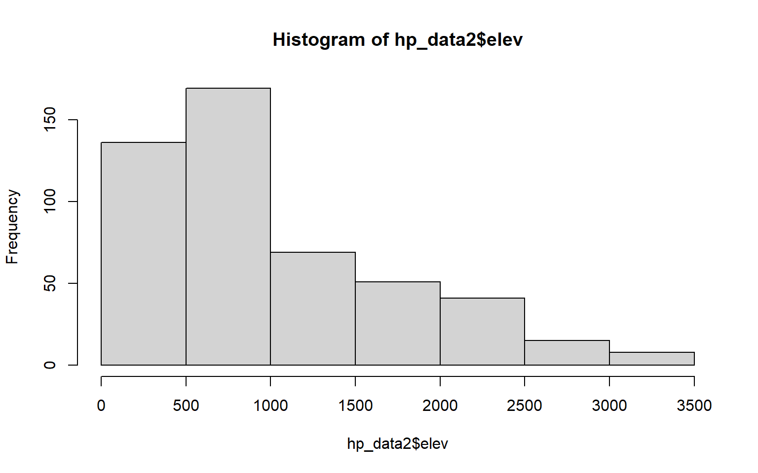
Summary Statistics by Group
As opposed to obtaining global summary statistics, you may be interested in summarizing data by group for comparison. The describeBy() function from the psych package expands upon describe() to allow for grouping. In the example below, I have obtained summary statistics by state. By default the result will be returned as a list object; however, you can set the mat argument to TRUE to obtain the output as a data frame.
for_stat <- describeBy(hp_data2$per_for, hp_data2$STATE_NAME, mat=TRUE)
print(for_stat)
    item       group1 vars   n      mean        sd     median    trimmed
X11    1     Colorado    1  64 18.341749 15.181901 22.7831594 17.9144943
X12    2       Kansas    1 105  2.769612  3.304699  1.4923449  2.2367985
X13    3      Montana    1  56 10.324312 10.899905  5.9975489  9.0668248
X14    4     Nebraska    1  93  1.294360  1.434022  0.8298879  1.0485710
X15    5 North Dakota    1  53  0.707462  1.087484  0.3632199  0.4430518
X16    6 South Dakota    1  66  1.495026  4.730695  0.3260004  0.4975848
X17    7         Utah    1  29 18.941720 10.148612 20.5519685 18.8203153
X18    8      Wyoming    1  23  6.201908  5.870400  4.6158960  5.4205776
           mad         min       max     range        skew   kurtosis        se
X11 19.0951614 0.001186869 44.739277 44.738091 -0.05466347 -1.5799113 1.8977377
X12  2.1437061 0.007282816 13.132781 13.125498  1.20217682  0.5142227 0.3225056
X13  8.0034310 0.027169554 34.771343 34.744174  0.86246043 -0.7133704 1.4565610
X14  1.0702851 0.006612731  6.504017  6.497405  1.42202432  1.4851247 0.1487012
X15  0.4160004 0.014679896  5.570716  5.556036  2.70381660  7.4230217 0.1493775
X16  0.3670117 0.004006820 33.882768 33.878761  5.43933498 31.9477734 0.5823083
X17 10.8379308 2.723746424 37.800489 35.076743 -0.01016540 -1.2541347 1.8845499
X18  4.4314006 0.179368100 25.384380 25.205012  1.49953605  2.4117033 1.2240631
Alternatively, you can use the dplyr group_by() function to obtain summary statistics by group. In the example below I am piping the data frame into group_by() followed by summarize() to obtain the mean county percent forest by state. If you would like to calculate a summary statistic for more than one column at once, you can use the summarize_all() function as opposed to summarize() as demonstrated in the second code block.
hp_data2 %>% group_by(STATE_NAME) %>% summarize(mn = mean(per_for))
# A tibble: 8 x 2
  STATE_NAME       mn
  <fct>         <dbl>
1 Colorado     18.3
2 Kansas        2.77
3 Montana      10.3
4 Nebraska      1.29
5 North Dakota  0.707
6 South Dakota  1.50
7 Utah         18.9
8 Wyoming       6.20
hp_data2 %>% group_by(STATE_NAME) %>% summarize_all(funs(mean))
# A tibble: 8 x 8
STATE_NAME NAME_1 TOTPOP10 POPDENS10 per_for temp elev precip2
<fct> <dbl> <dbl> <dbl> <dbl> <dbl> <dbl> <dbl>
1 Colorado NA 78581. 146. 18.3 6.85 2190. 5.14
2 Kansas NA 27173. 49.3 2.77 12.6 554. 7.58
3 Montana NA 17668. 7.35 10.3 5.80 1282. 4.73
4 Nebraska NA 19638. 42.3 1.29 9.82 694. 6.43
5 North Dakota NA 12690. 8.49 0.707 5.11 550. 4.68
6 South Dakota NA 12336. 14.0 1.50 7.72 596. 5.58
7 Utah NA 95306. 117. 18.9 8.27 1937. 4.39
8 Wyoming NA 24505. 6.37 6.20 5.88 1848. 4.14Statistical Methods
We will now explore some common statistical tests. Since this is not a statistics course, I will not demonstrate complex tests; however, if you need to conduct more complex tests than those demonstrated here, I think you will find that the syntax will be similar to the examples provided.
Correlation
The base R cor() function allows for the calculation of correlation between pairs of continuous variables. The following methods are available:
- Pearson Correlation Coefficient: parametric and assesses the linear correlation between two variables (similar to R-squared)
- Spearman’s Rank Correlation Coefficient: nonparametric measure of monotonic correlation based on ranks
- Kendal Rank Correlation Coefficient: nonparametric measure of monotonic correlation based on ranks and reported as probabilities
Parametric tests have assumptions relating to data distribution. For example, the data may be assumed to be normally distributed. If input data do not meet the distribution requirements, the tests may be invalid or misleading. In contrast, nonparametric tests do not have distribution assumptions and often rely on the ranks or order of data point values as opposed to their actual value or magnitude. They can serve as a more appropriate test when distribution assumptions are violated.
In the example below, I have compared the correlation between population density, percent forest cover, temperature, elevation, and precipitation using all three methods. Large positive values indicate direct or positive correlation between the two variables while negative values indicate indirect or inverse correlation between the two variables. You may have noticed that the diagonal values are 1 for all methods. This is because a variable is perfectly correlated with itself.
If you would like to visualize or graph variable correlations, I highly recommend the corrplot package.
cor(hp_data2[,4:8], method="pearson")
           POPDENS10     per_for       temp        elev    precip2
POPDENS10 1.00000000  0.01008319  0.1034935  0.03646341  0.0569110
per_for   0.01008319  1.00000000 -0.4199889  0.76004048  0.1356033
temp      0.10349346 -0.41998889  1.0000000 -0.52669255  0.4051434
elev      0.03646341  0.76004048 -0.5266925  1.00000000 -0.3306361
precip2   0.05691100  0.13560330  0.4051434 -0.33063615  1.0000000
cor(hp_data2[,4:8], method="spearman")
           POPDENS10    per_for       temp       elev    precip2
POPDENS10  1.0000000  0.2595500  0.2586090 -0.2622042  0.4927968
per_for    0.2595500  1.0000000 -0.2366128  0.2818702  0.2454769
temp       0.2586090 -0.2366128  1.0000000 -0.4462037  0.3763700
elev      -0.2622042  0.2818702 -0.4462037  1.0000000 -0.5538748
precip2    0.4927968  0.2454769  0.3763700 -0.5538748  1.0000000
cor(hp_data2[,4:8], method="kendall")
           POPDENS10    per_for       temp       elev    precip2
POPDENS10  1.0000000  0.1809036  0.1699107 -0.1929554  0.3508058
per_for    0.1809036  1.0000000 -0.1529384  0.1401321  0.1943746
temp       0.1699107 -0.1529384  1.0000000 -0.3186832  0.2619598
elev      -0.1929554  0.1401321 -0.3186832  1.0000000 -0.4153005
precip2    0.3508058  0.1943746  0.2619598 -0.4153005  1.0000000
T-Test
A T-test is used to statistically assess whether the means of two groups are different. The null hypothesis is that the means are not different, and the alternative hypothesis is that they are different. In the example, I first use dplyr to subset out only counties in Utah or North Dakota since we can only compare two groups with a T-test. Since statistical inference is used to infer something about a population from a sampled drawn from that population, I am also randomly sampling 15 counties from each of the two states. I also set a random seed so that the random sampling is reproducible. I then use the base R t.test() function to perform the test. Specifically, I assess whether the mean annual county temperatures are different for the two states. I provide a formula and a data set.
Once the test executes, the result will be printed to the console. A p-value of 0.000227 is obtained, which is much lower than 0.05. This indicates to reject the null hypothesis in favor of the alternative hypothesis that the average of mean annual temperature by county in these two states is different.
set.seed(42)
hp_sub <- hp_data2 %>% filter(STATE_NAME == "Utah" | STATE_NAME== "North Dakota") %>% group_by(STATE_NAME) %>% sample_n(15, replace=FALSE)t.test(temp ~ STATE_NAME, data=hp_sub)
Welch Two Sample t-test
data: temp by STATE_NAME
t = -3.7228, df = 18.688, p-value = 0.001477
alternative hypothesis: true difference in means is not equal to 0
95 percent confidence interval:
-4.015057 -1.123045
sample estimates:
mean in group North Dakota mean in group Utah
5.229322 7.798373 Mann-Whitney U Test
A T-test is a parametric test. As discussed above, this means that it has some assumptions. Specifically, the T-test assumes that the two groups are independent of each other, samples within groups are independent, the dependent variable is normally distributed, and the two groups have similar variance. It is likely that at least some of these assumptions are violated. For example, due to spatial autocorrelation, it is unlikely that samples are independent.
The Mann-Whitney U Test offers a nonparametric alternative to the T-test with relaxed distribution assumptions. However, it is still assumed that the samples are independent. The example below provides the result for the comparison of Utah and North Dakota. A statistically significant p-value is obtained, again suggesting a rejection of the null hypothesis in favor of the alternative hypothesis that the median of mean annual temperature by county is different between the two states.
wilcox.test(temp ~ STATE_NAME, data=hp_sub)

    Wilcoxon rank sum exact test

data:  temp by STATE_NAME
W = 43, p-value = 0.003155
alternative hypothesis: true location shift is not equal to 0
ANOVA
What if you would like to compare more than two groups? This can be accomplished using analysis of variance or ANOVA. There are many different types of analysis of variance that vary based on study design, such as One-Way ANOVA, Two-Way ANOVA, MANOVA, Factorial ANOVA, ANCOVA, and MANCOVA. Here, I will simply demonstrate One-Way ANOVA, which is used to compare the means of a single variable between groups. However, if you need to implement one of the more complex methods, you can use similar syntax.
Similar to the example above, I am assessing whether the mean annual temperature by county is different between states. However, now I am assessing all states in the data set as oppose to only two. Again, I subset out 15 counties for each state to represent a sample from the larger population. The null hypothesis is that no pair of means are different while the alternative hypothesis is that at least one pair of means is different. The test results in a statistically significant p-value, suggesting to reject the null hypothesis in favor of the alternative hypothesis that at least one pair of states have statistically different mean annual temperature by county. However, the test does not tell us what pair or pairs are different.
Following a statistically significant ANOVA result, it is common to use a pair-wise test to compare each pair combination. There are different methods available. Here, I am using the Tukey’s Honest Significant Difference method, made available by the TukeyHSD(), function to perform the comparisons. If the p-value is lower than 0.05 and the confidence interval does not include zero within its range, the states are suggested to be statistically significantly different at the 95% confidence level.
hp_dataSub2 <- hp_data2 %>% group_by(STATE_NAME) %>% sample_n(15, replace=FALSE)
fit <- aov(temp ~ STATE_NAME, data=hp_dataSub2)
summary(fit)
             Df Sum Sq Mean Sq F value Pr(>F)
STATE_NAME    7  612.3   87.47   26.27 <2e-16 ***
Residuals   112  372.9    3.33
---
Signif. codes:  0 '***' 0.001 '**' 0.01 '*' 0.05 '.' 0.1 ' ' 1
TukeyHSD(fit)
  Tukey multiple comparisons of means
    95% family-wise confidence level

Fit: aov(formula = temp ~ STATE_NAME, data = hp_dataSub2)

$STATE_NAME
                                 diff        lwr        upr     p adj
Kansas-Colorado            5.92144549  3.8631641  7.9797269 0.0000000
Montana-Colorado          -0.50712342 -2.5654048  1.5511580 0.9946954
Nebraska-Colorado          3.19839785  1.1401164  5.2566793 0.0001310
North Dakota-Colorado     -1.46578695 -3.5240684  0.5924945 0.3598855
South Dakota-Colorado      1.24441396 -0.8138675  3.3026954 0.5758138
Utah-Colorado              1.70734267 -0.3509387  3.7656241 0.1810802
Wyoming-Colorado          -0.47702519 -2.5353066  1.5812562 0.9963685
Montana-Kansas            -6.42856890 -8.4868503 -4.3702875 0.0000000
Nebraska-Kansas           -2.72304764 -4.7813291 -0.6647662 0.0020498
North Dakota-Kansas       -7.38723244 -9.4455139 -5.3289510 0.0000000
South Dakota-Kansas       -4.67703153 -6.7353129 -2.6187501 0.0000000
Utah-Kansas               -4.21410282 -6.2723842 -2.1558214 0.0000001
Wyoming-Kansas            -6.39847068 -8.4567521 -4.3401893 0.0000000
Nebraska-Montana           3.70552126  1.6472398  5.7638027 0.0000050
North Dakota-Montana      -0.95866353 -3.0169450  1.0996179 0.8371957
South Dakota-Montana       1.75153737 -0.3067440  3.8098188 0.1567801
Utah-Montana               2.21446608  0.1561847  4.2727475 0.0255972
Wyoming-Montana            0.03009823 -2.0281832  2.0883796 1.0000000
North Dakota-Nebraska     -4.66418480 -6.7224662 -2.6059034 0.0000000
South Dakota-Nebraska     -1.95398389 -4.0122653  0.1042975 0.0757472
Utah-Nebraska             -1.49105518 -3.5493366  0.5672262 0.3377195
Wyoming-Nebraska          -3.67542304 -5.7337045 -1.6171416 0.0000062
South Dakota-North Dakota  2.71020091  0.6519195  4.7684823 0.0021974
Utah-North Dakota          3.17312962  1.1148482  5.2314110 0.0001528
Wyoming-North Dakota       0.98876176 -1.0695197  3.0470432 0.8144071
Utah-South Dakota          0.46292871 -1.5953527  2.5212101 0.9969903
Wyoming-South Dakota      -1.72143915 -3.7797206  0.3368423 0.1730489
Wyoming-Utah              -2.18436786 -4.2426493 -0.1260864 0.0292465
Since ANOVA is a parametric method, it has assumptions, similar to the T-test. Specifically, ANOVA assumes that samples are independent, the data and model residuals (i.e., error terms) are normally distributed, and that variance is consistent between groups.
A Q-Q plot can be used to visually assess data normality by comparing the quantiles of the data to theoretical quantiles, or the quantiles the data would have if they were normally distributed. Divergence from the line suggests that the data are not normally distributed.
In the examples below I have created Q-Q plots using two different functions: qqnorm() and qqPlot(). The first plot represents the distribution of the temperature data while the second plot represents the distribution of the model residuals. Since the data points diverge from the line, this suggests that the data are not normally distributed and that an assumption of ANOVA is violated.
qqnorm(hp_dataSub2$temp)
qqline(hp_dataSub2$temp)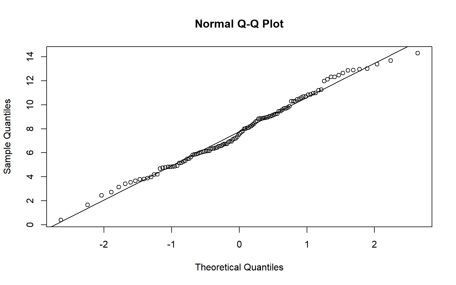
qqPlot(lm(temp~STATE_NAME, data=hp_dataSub2), simulate=TRUE, main="Q-Q Plot", labels=FALSE)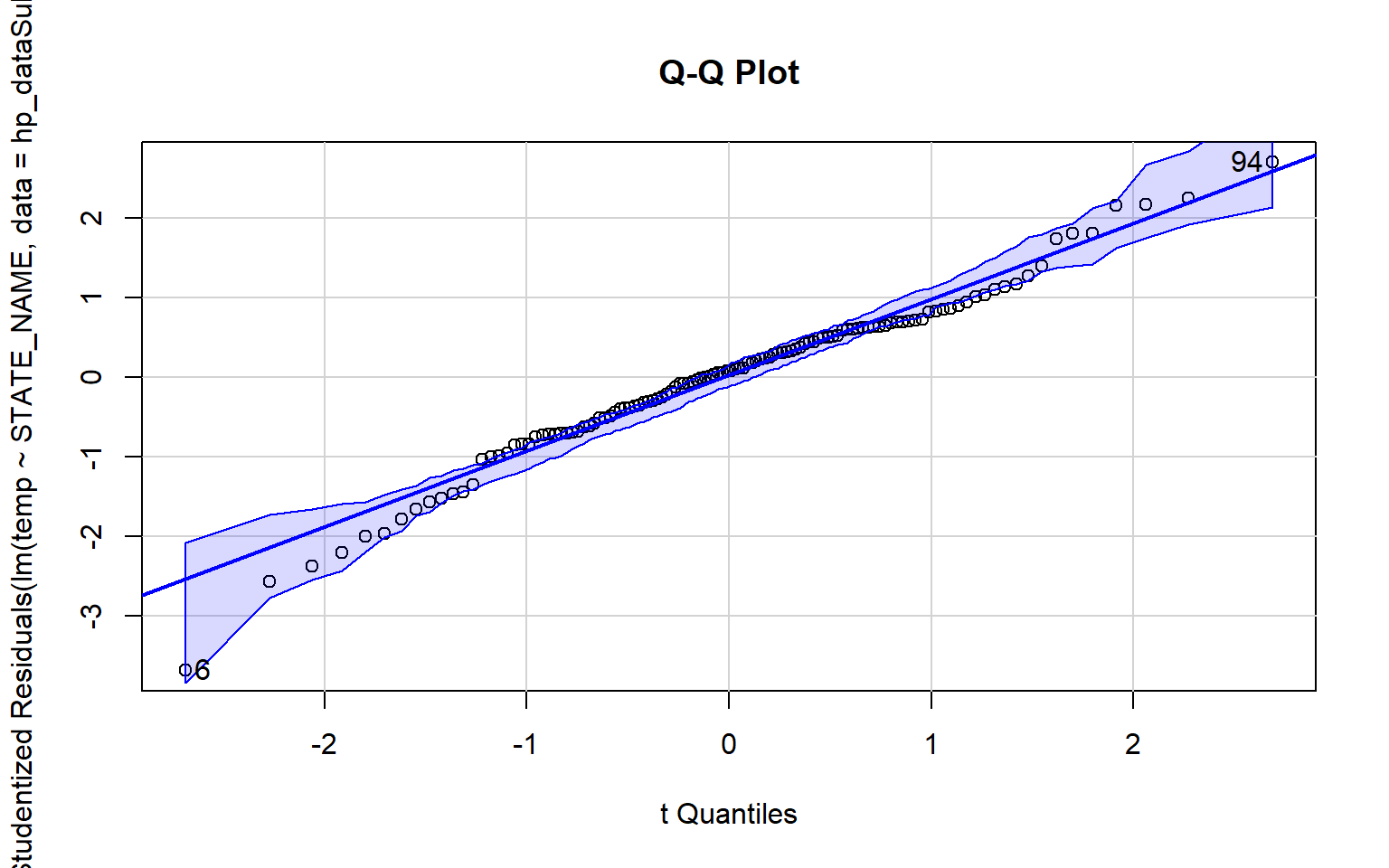
[1] 6 94The Bartlett Test of Homogeneity of Variance is used to assess whether variance is the same between groups. A statistically significant result, as obtained here, suggests that this assumption is violated.
bartlett.test(temp ~ STATE_NAME, data=hp_dataSub2)

    Bartlett test of homogeneity of variances

data:  temp by STATE_NAME
Bartlett's K-squared = 50.255, df = 7, p-value = 1.287e-08
ANOVA is also sensitive to outliers. The Bonferroni Outlier Test is used to determine whether outliers are present. The results in this case do suggest the presence of outliers.
outlierTest(fit)
   rstudent unadjusted p-value Bonferroni p
6 -3.685587         0.00035458      0.04255
Kruskal-Wallis Test
Since many of the assumptions of ANOVA are violated, as highlighted by the analysis above, it would be good to assess difference between groups using a nonparametric alternative. The Kruskal-Wallis Rank Sum Test provides this alternative. Similar to ANOVA, a statistically significant result, as obtained here, suggests that at least one pair of groups are different. It does not tell you what pair or pairs. So, I use the pairw.kw() function from the asbio package to perform a nonparametric pair-wise comparison. A p-value lower than 0.05 and a confidence interval that does not include zero in its range suggest difference between the two groups.
kruskal.test(temp ~ STATE_NAME, data=hp_data2)

    Kruskal-Wallis rank sum test

data:  temp by STATE_NAME
Kruskal-Wallis chi-squared = 367.65, df = 7, p-value < 2.2e-16
pairw.kw(hp_data2$temp, hp_data2$STATE_NAME, conf=0.95)

95% Confidence intervals for Kruskal-Wallis comparisons

                                Diff      Lower      Upper  Decision
Colorado-Kansas           -253.02917 -323.02863 -183.02971 Reject H0
Colorado-Montana            67.86607  -12.90254  148.63468    FTR H0
Kansas-Montana             320.89524  247.85532  393.93515 Reject H0
Colorado-Nebraska          -131.1539  -202.8432   -59.4646 Reject H0
Kansas-Nebraska            121.87527   59.02134   184.7292 Reject H0
Montana-Nebraska          -199.01997 -273.68094   -124.359 Reject H0
Colorado-North Dakota      102.26769     20.289  184.24638 Reject H0
Kansas-North Dakota        355.29686  280.92101   429.6727 Reject H0
Montana-North Dakota        34.40162  -50.18804  118.99128    FTR H0
Nebraska-North Dakota      233.42159  157.45318  309.38999 Reject H0
Colorado-South Dakota      -19.88068  -97.31718   57.55582    FTR H0
Kansas-South Dakota        233.14848  163.81111  302.48586 Reject H0
Montana-South Dakota       -87.74675 -167.94224   -7.55127 Reject H0
Nebraska-South Dakota      111.27322   40.23025  182.31618 Reject H0
North Dakota-South Dakota -122.14837 -203.56246  -40.73428 Reject H0
Colorado-Utah              -52.97629 -151.78346   45.83088    FTR H0
Kansas-Utah                200.05287  107.45634  292.64941 Reject H0
Montana-Utah              -120.84236 -221.82633   -19.8584 Reject H0
Nebraska-Utah                78.1776   -15.7029  172.05811    FTR H0
North Dakota-Utah         -155.24398 -257.19838  -53.28958 Reject H0
South Dakota-Utah          -33.09561 -131.43484   65.24362    FTR H0
Colorado-Wyoming            57.00272  -50.30765  164.31309    FTR H0
Kansas-Wyoming             310.03188  208.41113  411.65263 Reject H0
Montana-Wyoming            -10.86335 -120.18133   98.45462    FTR H0
Nebraska-Wyoming           188.15662   85.36455  290.94868 Reject H0
North Dakota-Wyoming       -45.26497 -155.48003   64.95008    FTR H0
South Dakota-Wyoming         76.8834  -29.99627  183.76307    FTR H0
Utah-Wyoming               109.97901  -13.26753  233.22555    FTR H0
                          Adj. P-value
Colorado-Kansas                      0
Colorado-Montana              0.242811
Kansas-Montana                       0
Colorado-Nebraska                    0
Kansas-Nebraska                      0
Montana-Nebraska                     0
Colorado-North Dakota         0.002729
Kansas-North Dakota                  0
Montana-North Dakota                 1
Nebraska-North Dakota                0
Colorado-South Dakota                1
Kansas-South Dakota                  0
Montana-South Dakota          0.017672
Nebraska-South Dakota          2.8e-05
North Dakota-South Dakota      7.8e-05
Colorado-Utah                        1
Kansas-Utah                          0
Montana-Utah                  0.005193
Nebraska-Utah                 0.260082
North Dakota-Utah              5.5e-05
South Dakota-Utah                    1
Colorado-Wyoming                     1
Kansas-Wyoming                       0
Montana-Wyoming                      1
Nebraska-Wyoming                     0
North Dakota-Wyoming                 1
South Dakota-Wyoming          0.689842
Utah-Wyoming                  0.148743
Concluding Remarks
Again, my goal here was to provide a demonstration of data summarization and statistical tests that can be performed in R. As this is not a statistics course, I did not explain the methods in detail or provide examples of more complex techniques. If you are interested in these topics, I would suggest taking a statistics course. If you need to perform more complex statistical analyses in R, you will find that they can be performed using similar syntax to the examples provided here.
We will discuss more data summarization in later modules including data visualization and graphing with ggplot2. In regards to statistical methods, we will explore linear regression and machine learning later in the course.