Raster Analysis with terra
Raster Analysis with terra
Objectives
- Get started using the terra package for working with geospatial data
- Work with the geospatial classes introduced by terra
- Perform raster preprocessing, math, and overlay tasks
- Work with remotely sensed data
- Perform supervised classification of raster data
Overview
In this module, we will focus on the terra package, which is replacing the raster package for working with raster-based geospatial data. The raster package has been a central tool for working with geospatial data in R for years. However, recently the originators of raster have released the terra package to replace raster. The raster package can be slow and can result in memory issues if large raster datasets are used. terra works to alleviate some of these issues. First, it is very fast since it makes use of C++ code. It also supports working with larger data sets as it is not required to read entire raster grids into memory.
Here are some helpful links for learning terra:
The terra package introduces the following new classes:
- SpatRaster: for raster data and limits memory usage in comparison to the raster package data models
- SpatVector: represent vector-based point, line, or polygon features and their associated attributes
- SpatExtent: for spatial extent information derived from a SpatRaster or SpatVector or manually defined
Although we will not explore it directly here, the stars package offers additional functionality to efficiently work with spatial data including spatiotemporal arrays, raster data cubes, and vector data cubes. The documentation for this package is available here.
The link at the bottom of the page provides the example data and R Markdown file used to generate this module.
Creating and Reading Data
Build a spatRaster from Scratch
First, I read in the required packages. Note that terra relies on C++, so you need to have the Rcpp package installed, which allows for R and C++ integration.
library(terra)
library(tmap)
library(tmaptools)
library(sf)
library(dplyr)
library(randomForest)
library(ggplot2)
library(RColorBrewer)
library(RStoolbox)
library(yardstick)
Using terra, all raster grids, regardless of the number of bands included, are created or read in as spatRaster objects using the rast() function. This is in contrast to the raster package, in which several functions are used. Specifically, the raster() function is used to read in single band data while the brick() function is used to read in multiband data. The stack() function can be used to reference multiple files as a single object. In short, terra simplifies the reading of raster data by using a single function.
In the following code block, I first create a raster grid by defining the number of rows, columns, min/max coordinates, and spatial reference information. The spatial reference information is defined using a European Petroleum Survey Group, or EPSG, code. By simply calling the spatRaster using its name, information about the object is returned. The spatial resolution is 10-by-10 meters, which is the cell size required to fill the defined spatial extent with the number of specified rows and columns.
#Build raster data from scratch
basic_raster <- rast(ncols = 10, nrows = 10, xmin = 500000, xmax = 500100, ymin = 4200000, ymax = 4200100, crs="+init=EPSG:26917")
basic_raster
class       : SpatRaster
dimensions  : 10, 10, 1  (nrow, ncol, nlyr)
resolution  : 10, 10  (x, y)
extent      : 5e+05, 500100, 4200000, 4200100  (xmin, xmax, ymin, ymax)
coord. ref. : NAD83 / UTM zone 17N
The raster I created above does not actually have any values stored in or associated with each cell. So, I next fill the grid with random values between 0 and 255 to simulate a 8-bit unsigned, single band dataset. I then plot the resulting grid using the tmap package. terra has a plot() function for visualizing single band raster data; however, I prefer to use tmap. Note that you will get different values than I did since the values are randomly generated.
vals <- sample(c(0:255), 100, replace=TRUE)

values(basic_raster) <- vals

tm_shape(basic_raster)+
  tm_raster()+
  tm_layout(legend.outside = TRUE)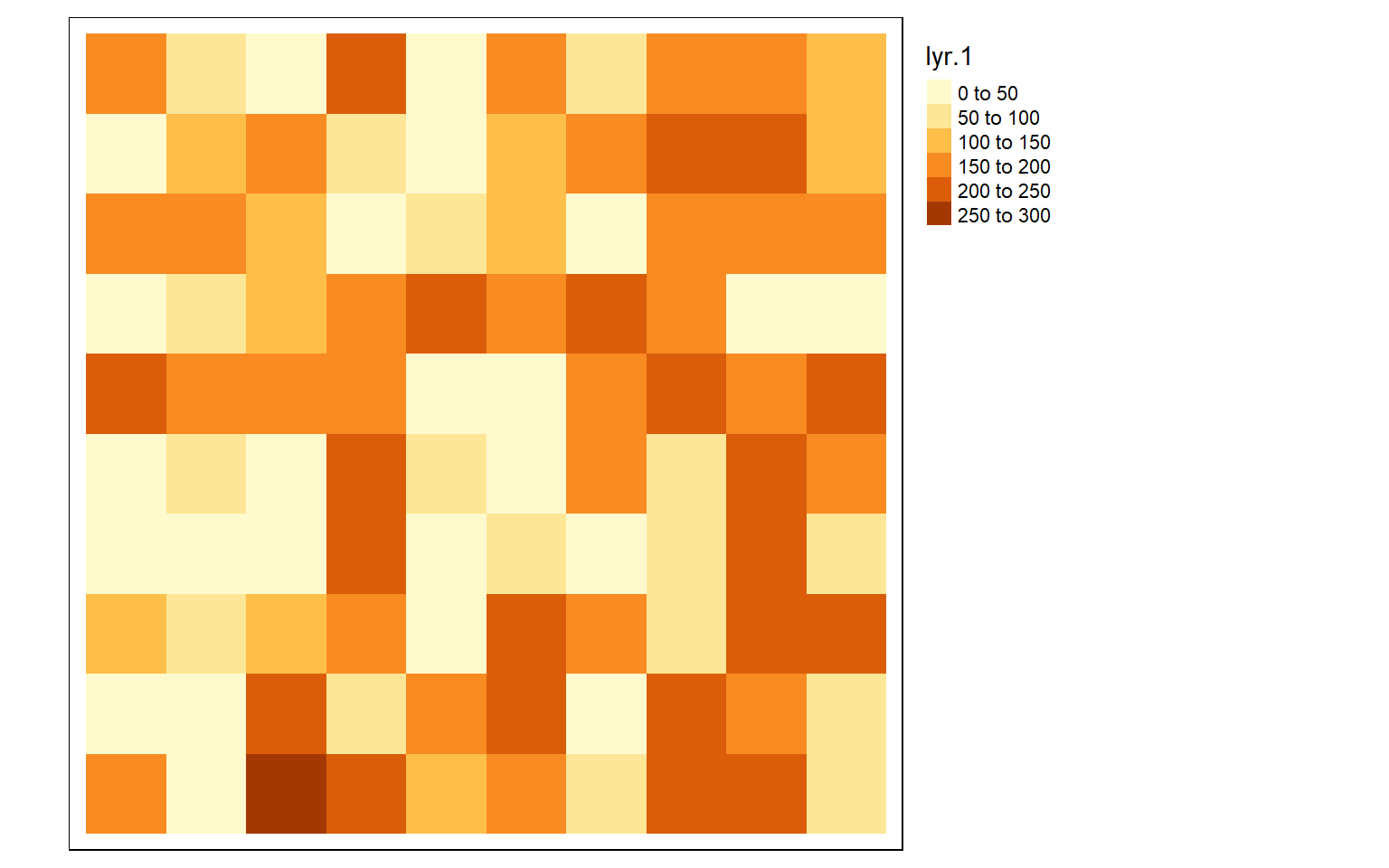
Reading Raster Data
Instead of generating a spatRaster object from scratch, you will likely want to read in data from an existing file. This can be accomplished using the rast() function and the associated file path and file name. First, I read in a digital elevation model, or DEM, obtained from the United States Geological Survey (USGS) National Elevation Dataset (NED) and plot it using tmap. I will provide a review of tmap below.
#Read in single-band data
dem <- rast("C:/terraWS/canaan/dem_example.tif")

tm_shape(dem)+
  tm_raster(style= "cont", palette=get_brewer_pal("-Greys", plot=FALSE))+
  tm_layout(legend.outside = TRUE)
Next, I read in a categorical raster of land cover, which is a subset of the National Land Cover Database (NLCD). Since this is a categorical raster, I display it using unique colors and provide names for each category, which are represented as numeric codes in the raster data.
lc <- rast("C:/terraWS/canaan/lc_example.tif")

tm_shape(lc)+
  tm_raster(style= "cat",
            labels = c("Open Water", "Developed Open", "Developed Low Int.", "Developed Med. Int.", "Developed High Int.", "Barren", "Deciduous Forest", "Evergreen Forest", "Mixed Forest", "Pasture/Hay", "Cultivated Crop", "Woody Wetland", "Emergent Wetland"),
            palette = c("deepskyblue", "brown1", "brown2", "brown3", "brown4", "darkgrey", "darkolivegreen", "darkolivegreen1", "darkseagreen1", "goldenrod3", "darkorange", "darkorchid1", "darkorchid4"),
            title="Land Cover")+
  tm_layout(legend.outside = TRUE)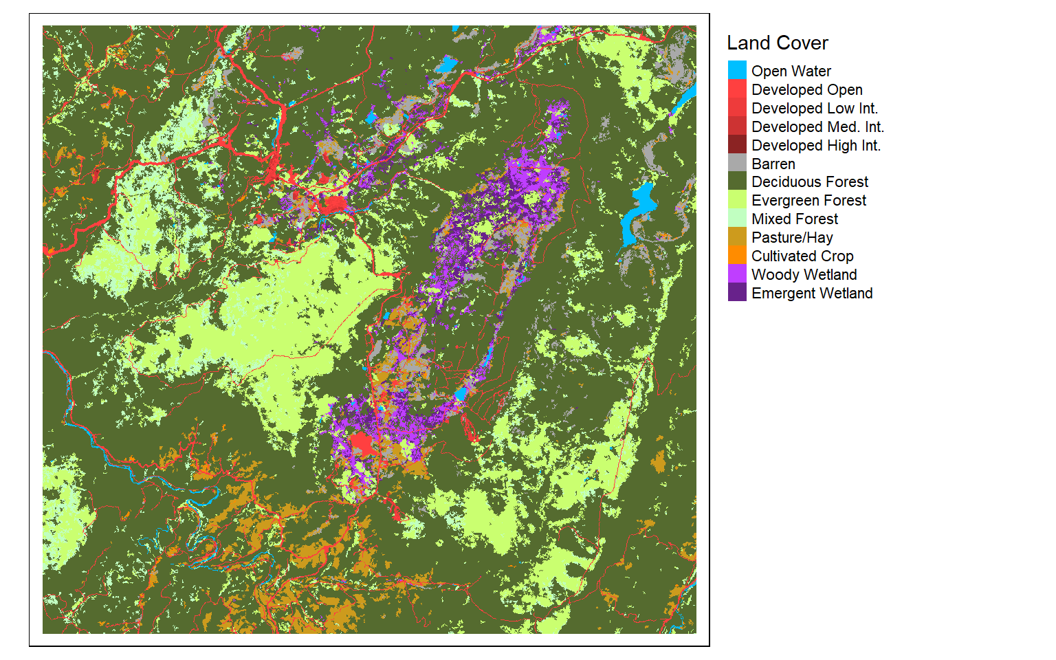
Reading in multiband raster data is not different from reading in single band data; you still use the rast() function. In the example below I am reading in a Sentinel-2 Multispectral Instrument (MSI) image from the European Space Agency (ESA) for the area around Vancouver, British Columbia, Canada. To display the multiband image as a false color composite, I use the plotRGB() function from terra; map bands to the red, green, and blue color channels; and apply a linear stretch. Here, I am mapping the near infrared (NIR) band to the red channel, red to green, and green to blue. In the next block of code, I map the SWIR1 band to red, NIR to green, and green to blue. The plotRGB() function provides options for applying a linear stretch (“lin”) or histogram equalization (“hist”). You can also change the extent to zoom in or out, map a color to NA pixels, and apply transparency.
s2 <- rast("C:/terraWS/vancouver/sentinel_vancouver.tif")

plotRGB(s2, r=4, g=3, b=2, stretch="lin")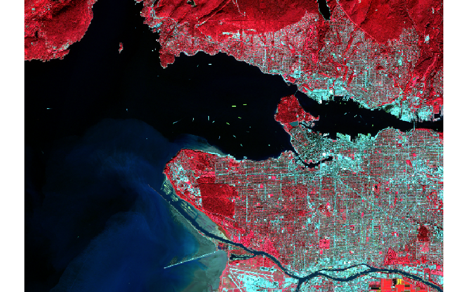
plotRGB(s2, r=5, g=4, b=2, stretch="lin")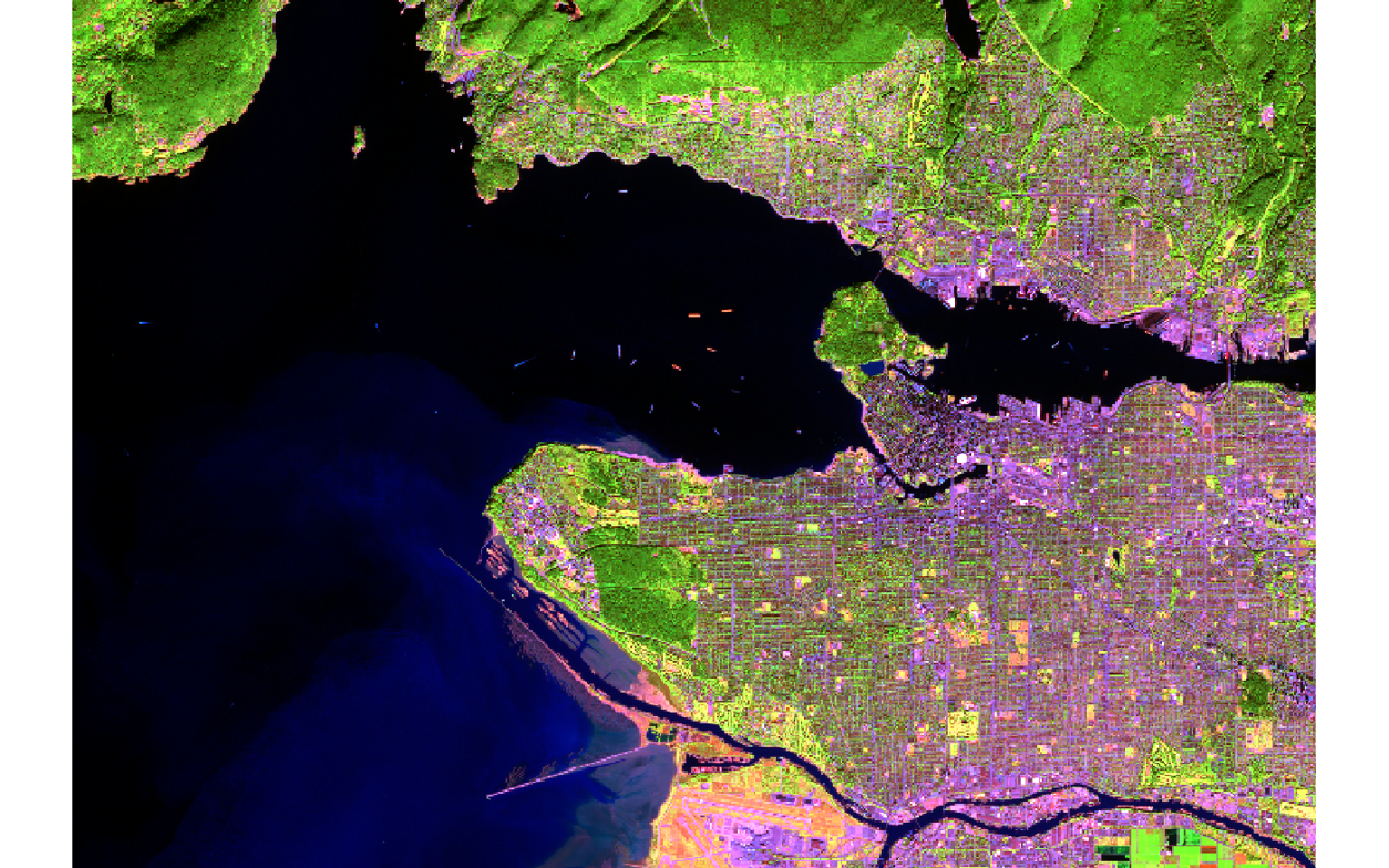
As mentioned above, simply calling the spatRaster object using its variable name will return information about the data. There are also a variety of additional functions to obtain certain pieces of information about the data. For example, ncol() returns the number of columns, nrow() returns the number of rows, ncell() returns the number of cells (rows X columns), and nlyr() returns the number of layers or bands. The res() function provides the resolution of the data relative to the units of the map projection, in this case meters. The names assigned to each band can be obtained using the names() function. Lastly, inMemory() will return Boolean TRUE or FALSE depending on whether or not the data are stored in memory or RAM.
ncol(s2)
[1] 2902
nrow(s2)
[1] 2026
ncell(s2)
[1] 5879452
nlyr(s2)
[1] 6
res(s2)
[1] 10 10
names(s2)
[1] "sentinel_vancouver_1" "sentinel_vancouver_2" "sentinel_vancouver_3"
[4] "sentinel_vancouver_4" "sentinel_vancouver_5" "sentinel_vancouver_6"
inMemory(s2)
[1] FALSE
You can also use these functions to change the attributes of the spatRaster. In the code cell below, I am changing the names assigned to each band.
names(s2) <- c("blue", "green", "red", "nir", "swir1", "swir2")
names(s2)
[1] "blue"  "green" "red"   "nir"   "swir1" "swir2"
Before moving on, I want to provide a few notes about the spatExtent class. This class is used to define the geographic extent (maximum and minimum X and Y values) for a data layer. Below, I have used the ext() function to extract the spatial extent of the Sentinel-2 image of Vancouver relative to the associated map projection, in this case UTM Zone 10N as easting and northing in meters. You can obtain or set the coordinate reference system or map projection information using the crs() function. Note that the crs() function only changes the projection associated with the data; it does not actually reproject coordinates. To reproject the data to a new coordinate reference system, you must use the project() function, which requires defining the desired reference system using another spatRaster object’s coordinate reference system information or defining the projection information using well known text (WKT), a PROJ.4 string, or an EPSG code. Note that PROJ.4 is now deprecated except for WGS84/NAD83 and NAD27 datums.
s2Ext <- ext(s2)
s2Ext
SpatExtent : 471120, 500140, 5448630, 5468890 (xmin, xmax, ymin, ymax)
Visualizing Raster Data
Before further discussing terra, I want to provide some background on how to visualize raster geospatial data in R. This is a bit of a review of the tmap module. As noted above, in terra single band images can be visualized using the plot() function while multiband images can be visualized using plotRGB(). In this workshop, I will use plotRGB() to display multispectral data. However, I prefer using tmap to visualize single band data. So, I will provide some background here on using tmap to display raster data. We will not discuss other components of this package, such as displaying vector data and making map layouts. Feel free to review the tmap module or a more detailed refresher.
In tmap, single-band raster data are symbolized using tm_raster() as demonstrated in the next code block. This is a DEM, which is a continuous raster.
tm_shape(dem)+
tm_raster()+
tm_layout(legend.outside = TRUE)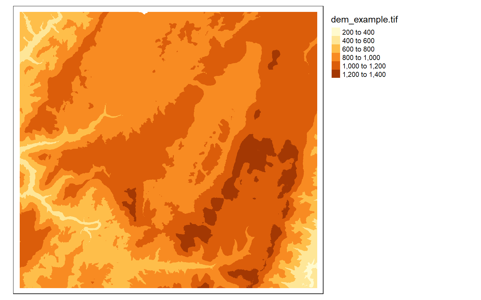
Similar to most GIS software packages, data values can be grouped or binned to represent a range of values with one color. Some common methods used include the following:
- Equal Interval: equal range of data values in each bin
- Quantiles: equal number of map features or grid cells in each bin
The next two examples demonstrate these different classification schemes.
tm_shape(dem)+
tm_raster(style= "equal")+
tm_layout(legend.outside = TRUE)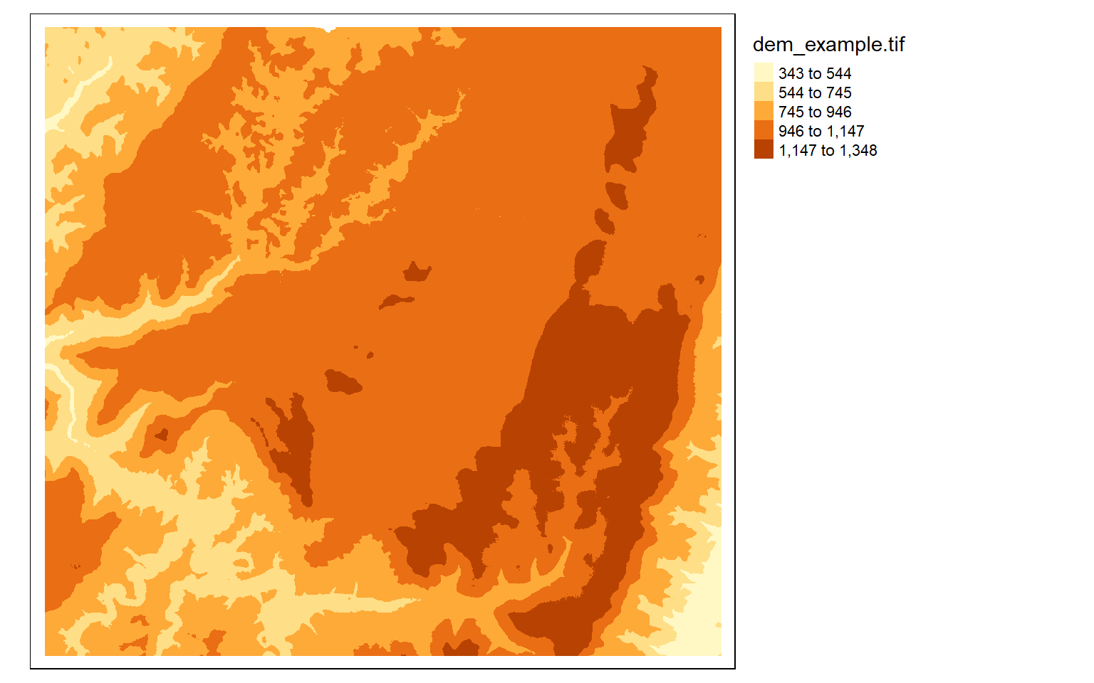
tm_shape(dem)+
tm_raster(style= "quantile")+
tm_layout(legend.outside = TRUE)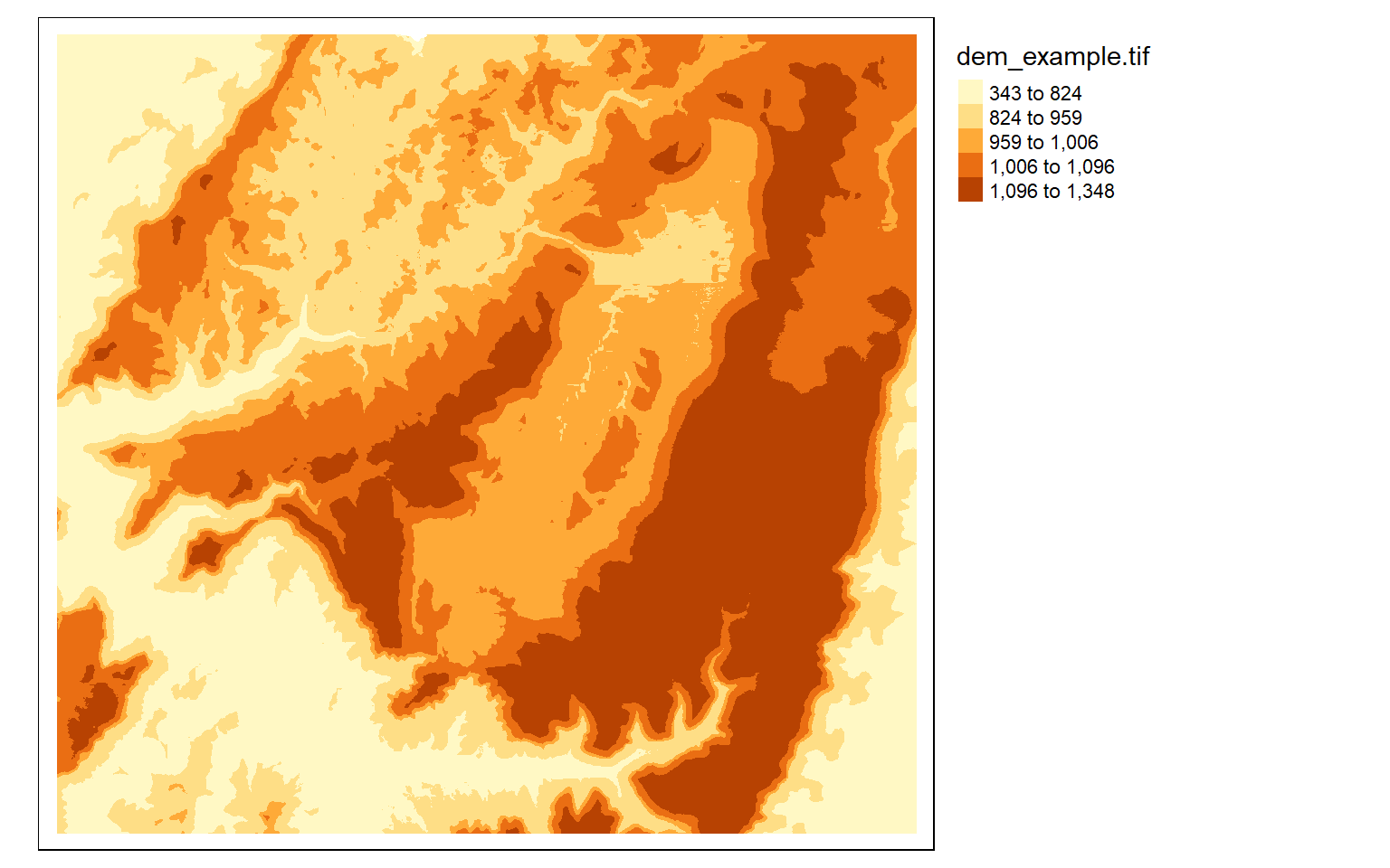
If you do not want to group colors into ranges or bins, you can use the continuous method where a color ramp is used to display the data without binning.
tm_shape(dem)+
tm_raster(style= "cont")+
tm_layout(legend.outside = TRUE)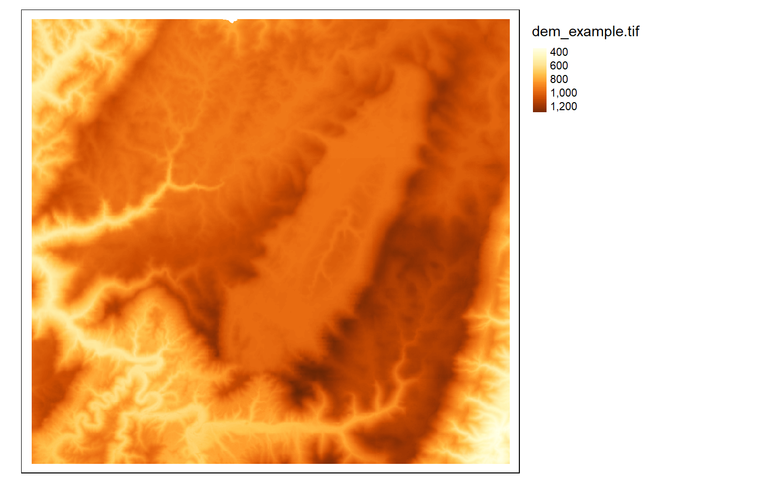
The next set of examples demonstrate applying ColorBrewer2 color palettes via the RColorBrewer package. Note that these ramps can be applied when using classified or continuous visualization methods.
tm_shape(dem)+
tm_raster(style= "quantile", n=7, palette=get_brewer_pal("Blues", n = 7, plot=FALSE))+
tm_layout(legend.outside = TRUE)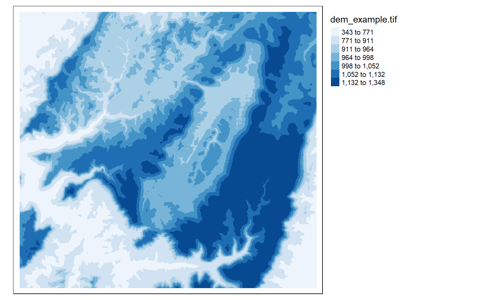
tm_shape(dem)+
tm_raster(style= "quantile", n=7, palette=get_brewer_pal("Greys", n = 7, plot=FALSE))+
tm_layout(legend.outside = TRUE)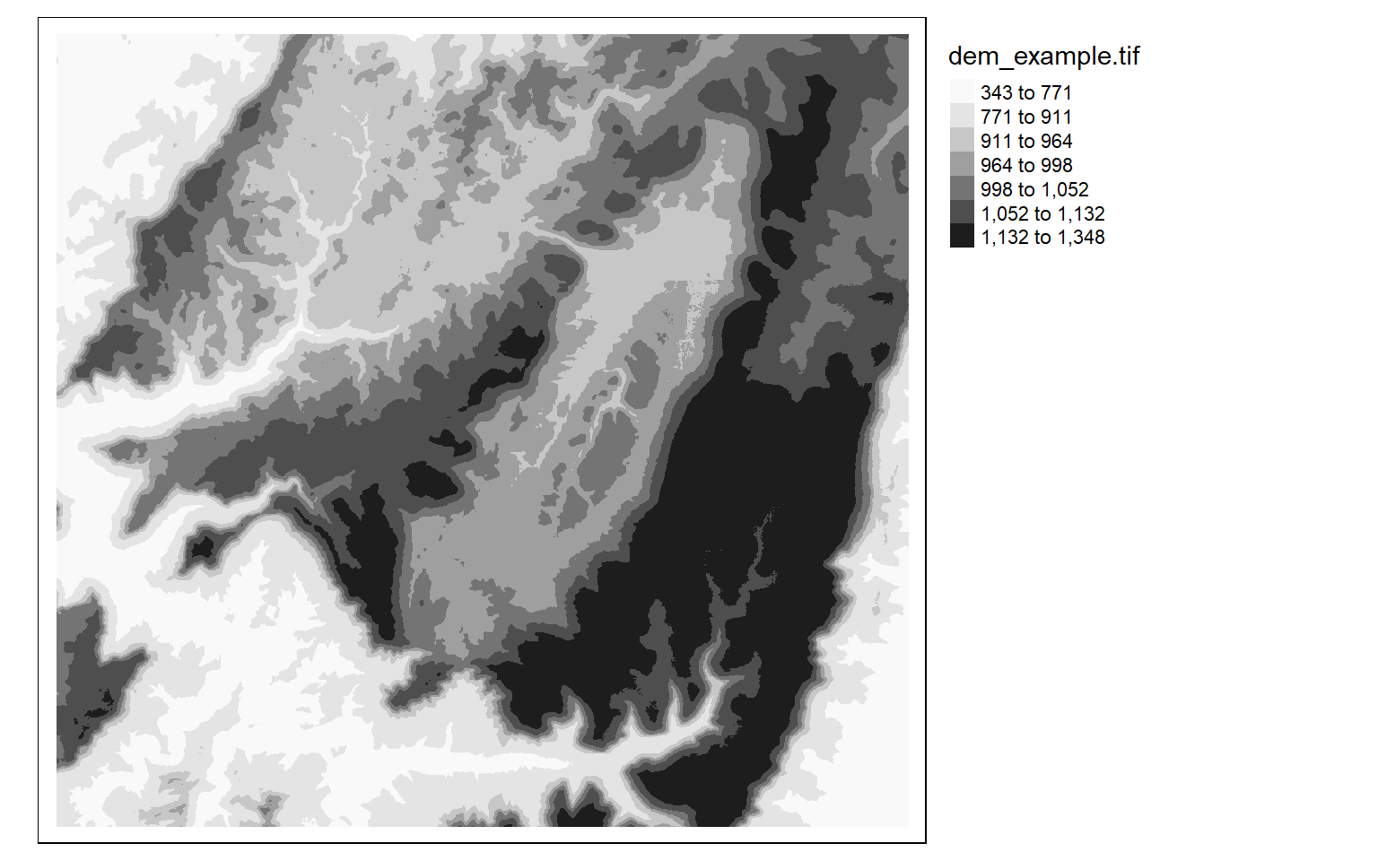
tm_shape(dem)+
tm_raster(style= "cont", palette=get_brewer_pal("Greys", plot=FALSE))+
tm_layout(legend.outside = TRUE)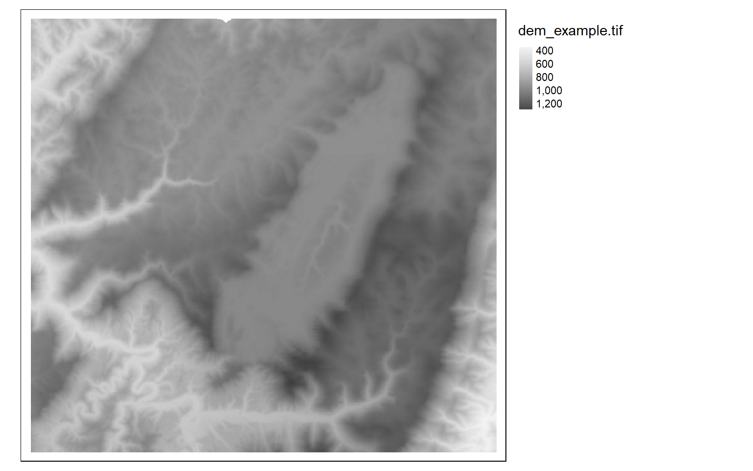
It is also possible to invert the color ramp by adding a negative sign to the name.
tm_shape(dem)+
tm_raster(style= "cont", n=7, palette=get_brewer_pal("-Greys", plot=FALSE))+
tm_layout(legend.outside = TRUE)
Now we will investigate symbolizing categorical raster data. This can be accomplished by setting the style argument equal to “cat.”
tm_shape(lc)+
tm_raster(style= "cat", title="Land Cover")+
tm_layout(legend.outside = TRUE)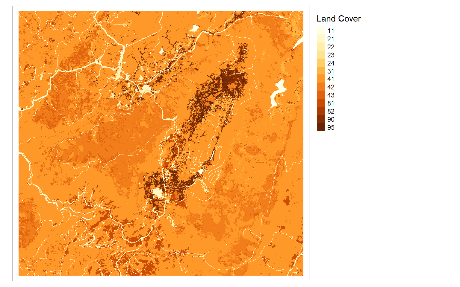
I generally find that I need to provide my own labels and colors for categorical data. In this example, I provide labels for each code so that the land cover category is displayed as opposed to the stand-in cell value. I also provide my own color palette using named R colors. Similar to ggplot2, the codes, labels, and colors must be in the same order so that they match up correctly, since this is based on the position or index only. Note that you could also provide hex codes or RGB values to define desired colors.
tm_shape(lc)+
tm_raster(style= "cat",
labels = c("Open Water", "Developed Open", "Developed Low Int.", "Developed Med. Int.", "Developed High Int.", "Barren", "Deciduous Forest", "Evergreen Forest", "Mixed Forest", "Pasture/Hay", "Cultivated Crop", "Woody Wetland", "Emergent Wetland"),
palette = c("deepskyblue", "brown1", "brown2", "brown3", "brown4", "darkgrey", "darkolivegreen", "darkolivegreen1", "darkseagreen1", "goldenrod3", "darkorange", "darkorchid1", "darkorchid4"),
title="Land Cover")+
tm_layout(legend.outside = TRUE)
Raster Preprocessing
Crop, Mask, and Merge
We will now explore some common raster preprocessing operations as implemented in terra. To demonstrate, I am reading in a digital elevation model from NED for a portion of the state of West Virginia.
elev <- rast("C:/terraWS/wv/elevation1.tif")

tm_shape(elev)+
  tm_raster(style= "cont")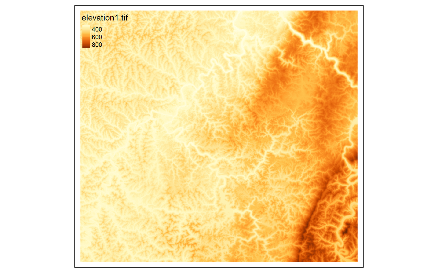
A rectangular extent can be extracted from a larger dataset using the crop() function and providing a desired extent defined using the xmin, xmax, ymin, and ymax coordinates relative to the map projection as a spatExtent object defined using the ext() function. In order to crop a raster relative to a rectangular extent or bounding box of another geospatial layer, you can use the extent of that layer in the crop operation as demonstrated in the following code block. In the example, I am using the spatial extent of a watershed boundary, read in as a spatVector object. Note that I have found that spatVector objects cannot be plotted with tmap, so I also read in the data as an sf object using the sf package.
crop_extent <- ext(580000, 620000, 4350000, 4370000)
elev_crop <- crop(elev, crop_extent)

tm_shape(elev_crop)+
  tm_raster(style= "cont")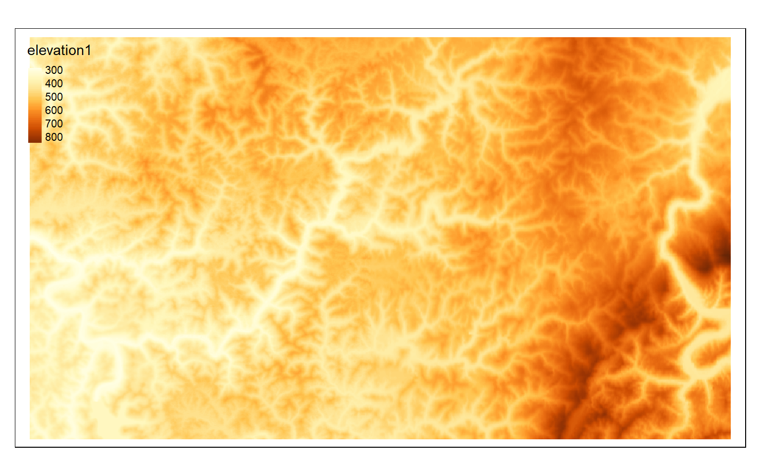
ws <- st_read("C:/terraWS/wv/watersheds.shp")
Reading layer `watersheds' from data source `C:\terraWS\wv\watersheds.shp' using driver `ESRI Shapefile'
Simple feature collection with 11 features and 15 fields
Geometry type: POLYGON
Dimension:     XY
Bounding box:  xmin: 554473.9 ymin: 4337973 xmax: 610447.8 ymax: 4389046
Projected CRS: WGS 84 / UTM zone 17N
ws2 <- vect("C:/terraWS/wv/watersheds.shp")
elev_crop2 <- crop(elev, ext(ws2))

tm_shape(elev_crop2)+
  tm_raster(style= "cont")+
  tm_shape(ws)+
  tm_borders(col="black")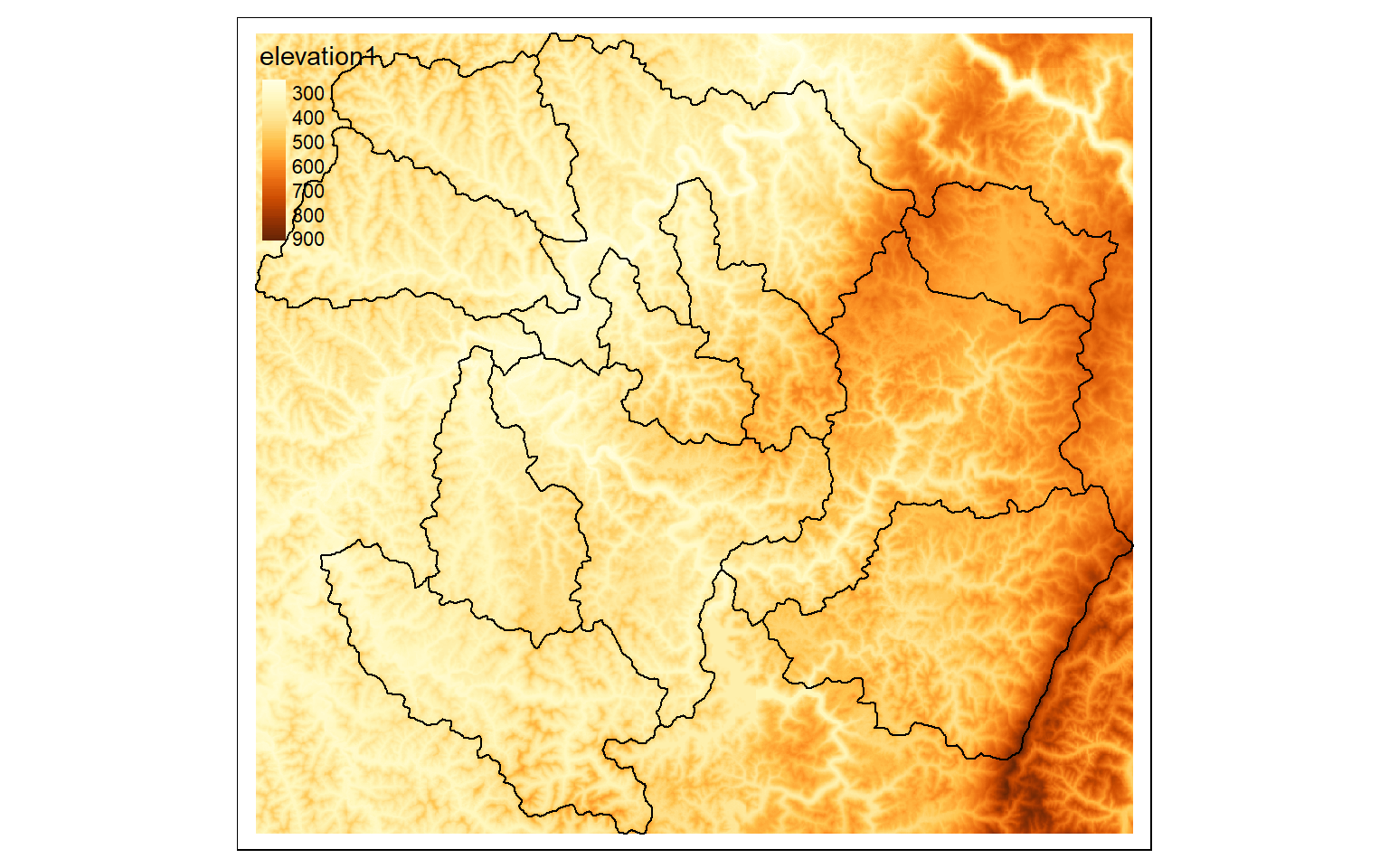
If you want to mask out cells that are not within an extent, as opposed to cropping relative to a rectangular extent, you can use the mask() function and specifying the desired mask as a spatRaster or spatVector object. Since all raster data must be rectangular, the cells outside of the masked extent still exist but now hold a NULL or NA assignment, which can be displayed using the colorNA argument of tm_raster() in tmap, as demonstrated in the second code block.
ws <- st_read("C:/terraWS/wv/watersheds.shp")
Reading layer `watersheds' from data source `C:\terraWS\wv\watersheds.shp' using driver `ESRI Shapefile'
Simple feature collection with 11 features and 15 fields
Geometry type: POLYGON
Dimension:     XY
Bounding box:  xmin: 554473.9 ymin: 4337973 xmax: 610447.8 ymax: 4389046
Projected CRS: WGS 84 / UTM zone 17N
ws2 <- vect("C:/terraWS/wv/watersheds.shp")
elev_mask <- mask(elev, ws2)

tm_shape(elev_mask)+
  tm_raster(style= "cont")+
  tm_shape(ws)+
  tm_borders(col="black")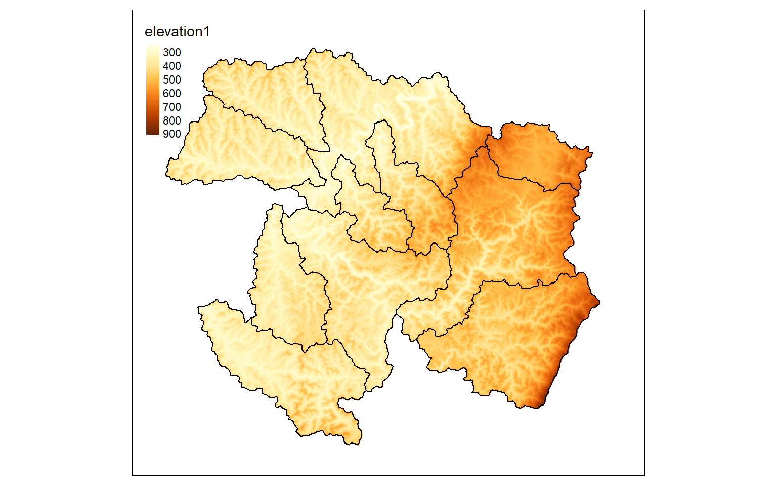
tm_shape(elev_mask)+
  tm_raster(style= "cont", colorNA="pink")+
  tm_shape(ws)+
  tm_borders(col="black")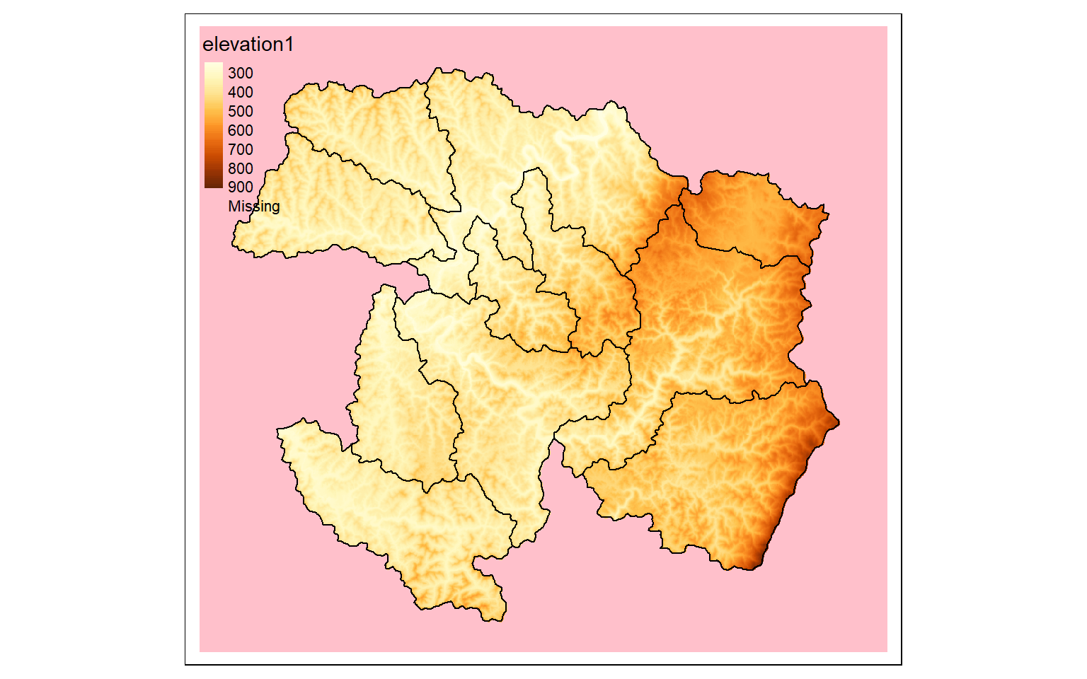
The merge() function is used to merge two spatRasters to a single raster. To demonstrate, I have extracted a second extent from the larger dataset then merged it with the subset created above.
elev_crop3 <- crop(elev, ext(570000,600000, 432000,4360000))

#Merge cropped extents
elev_merge <- terra::merge(elev_crop, elev_crop3)

tm_shape(elev_merge)+
  tm_raster(style= "cont")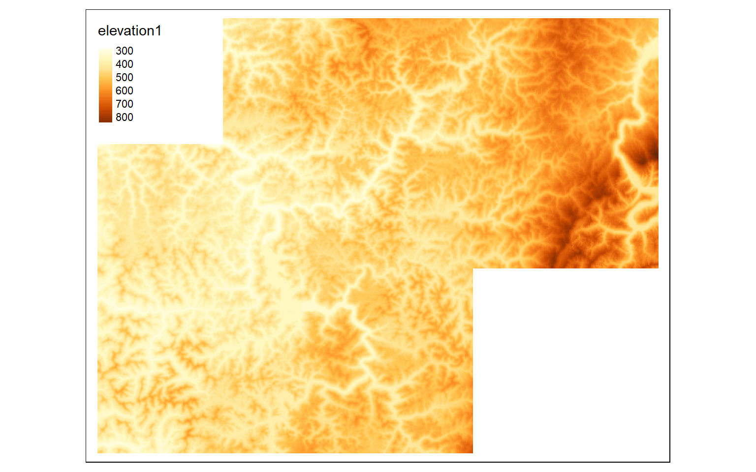
Aggregate and Resample
The aggregate() function is used to combine adjacent cells into a single cell, effectively degrading the raster to a coarser cell size. This is demonstrated below where an original grid that has a cell size of 30-by-30 meters is aggregated by a factor of five to obtain a new grid with a cell size of 150-by-150 meters. The fun argument determines how the new value in the cell is calculated from the original cells. In this example, I return the mean of the original values in the cell.
terra is less forgiving in regards to differences in origin and spatial extent when performing raster overlay. So, it is generally necessary to make sure all input data have the same origin and spatial extent so that the cells align. One means to do this is to use the resample() function to align one spatRaster object with another object. This function provides several resampling methods including nearest neighbor, bilinear interpolation, cubic interpolation, cubic spline interpolation, and Lanczos windowed sinc. So, resample(), similar to aggregate(), can also be used to change the cell size of a raster grid and is particularly useful when you want to align grids to a common origin and extent.
elev_agg <- aggregate(elev, fact=5, fun=mean)
elev_agg
class       : SpatRaster
dimensions  : 385, 423, 1  (nrow, ncol, nlyr)
resolution  : 150, 150  (x, y)
extent      : 551467.6, 614917.6, 4335125, 4392875  (xmin, xmax, ymin, ymax)
coord. ref. : WGS_1984_UTM_Zone_17N (EPSG:32617)
source(s)   : memory
name        : elevation1
min value   :      242.0
max value   :      955.2
Subset and Stack Bands
The subset() function is used to extract bands from a spatRaster into a new spatRaster while the c() function is used to combine bands from multiple spatRaster objects into a new, multiband spatRaster. Note that the band names are maintained, as demonstrated in the code block below.
The second code block demonstrates other methods to subset bands from a spatRaster using band names and indexing.
s2Vis <- subset(s2, c(1,2,3))
s2NIR <- subset(s2, 4)
s2SWIR <- subset(s2, c(5,6))

s2VisNIR <- c(s2Vis, s2NIR)

names(s2Vis)
[1] "blue"  "green" "red"
names(s2NIR)
[1] "nir"
names(s2SWIR)
[1] "swir1" "swir2"

names(s2VisNIR)
[1] "blue"  "green" "red"   "nir"
s2Red <- s2$red
names(s2Red)
[1] "red"
s2SWIR <- s2[[5:6]]
names(s2SWIR)
[1] "swir1" "swir2"Reclassify
It is possible to change the cell values for categorical or continuous raster data using reclassification as implemented by the classify() function in terra. This requires that a table be generated to define the ranges of values to reclassify and the associated new cell value or code. In the first example below, I have classified the elevation data into bins by (1) creating a vector of values, (2) creating a three-column matrix from this vector, and (3) using the classify() function. Note that the right argument determines how boundary conditions are handled. If it is set to TRUE the intervals are closed to the right and open to the left (i.e., the high value is included in the interval but the low value is not). If FALSE the interval is open to the right and closed to the left (low value is included but high value is not). In contrast, “open” means that the extreme values, high and low, are not included in the interval. It is also possible to close both sides with right=NA.
As noted above, in the first example below, I am reclassifying a continuous grid using a three-column matrix of “from”, “to”, and “becomes” columns. In the next example, I am reclassifying a categorical land cover grid using a two-column matrix representing “old” and “new” categories. Specifically, forest categories are coded to 1 and all other categories are coded to 0 to created a binary forest vs. not forest dataset.
m <- c(0, 300, 1,  300, 500, 2,  500,
       800,  3, 800, 10000, 4)
m <- matrix(m, ncol=3, byrow = TRUE)

dem_re <- classify(elev, m, right=TRUE)

tm_shape(dem_re)+
  tm_raster(style= "cat")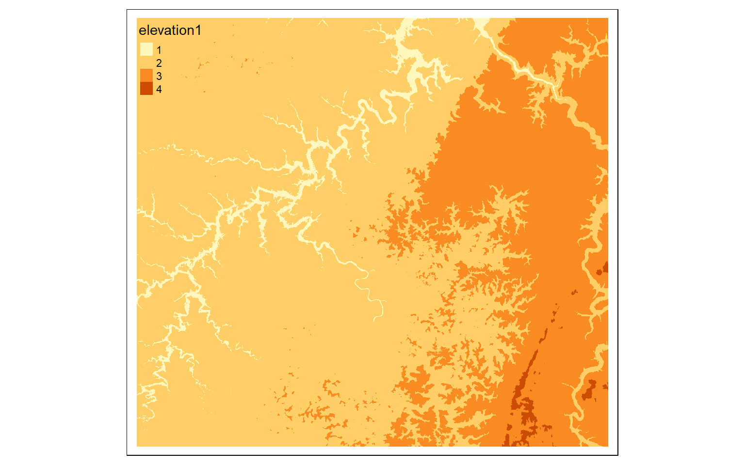
m2 <- c(11, 0, 21, 0, 22, 0, 23, 0, 24, 0, 31, 0, 41, 1, 42, 1, 43, 1, 51, 0, 52, 0, 71, 0, 72, 0, 73, 0, 74, 0, 81, 0, 82, 0, 90, 1, 95, 0)
m2 <- matrix(m2, ncol=2, byrow = TRUE)

lc_re <- classify(lc, m2, right=TRUE)

tm_shape(lc_re)+
  tm_raster(style= "cat", labels = c("Not Forest", "Forest"), palette = c("gray", "darkolivegreen"))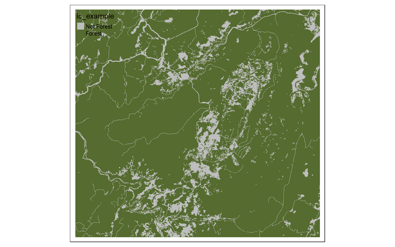
General Raster Analysis
We will now explore a variety of common raster analysis tasks that are traditionally performed using GIS software.
Raster Summarization
The extract() function can be used to extract cell values at point locations or obtain statistics within polygon or categorical raster grid extents. In the first example below, I am extracting out elevation values at point locations. The result is a data frame, or table, object. I then merge the results back onto the point features represented as an sf object to plot them.
In the second example, I obtain the mean elevation by watershed by extracting values by polygon extents as opposed to point locations. Different statistics can be obtained by changing the fun argument.
pnts <- st_read("C:/terraWS/wv/example_points.shp")
Reading layer `example_points' from data source `C:\terraWS\wv\example_points.shp' using driver `ESRI Shapefile'
Simple feature collection with 47 features and 1 field
Geometry type: POINT
Dimension:     XY
Bounding box:  xmin: 556505.6 ymin: 4341385 xmax: 608028.9 ymax: 4388863
Projected CRS: WGS 84 / UTM zone 17N

pnts2 <- vect("C:/terraWS/wv/example_points.shp")

pnts_elev <- terra::extract(elev, pnts2)
pnts_elev2 <- pnts_elev

pnts$elev <- as.numeric(pnts_elev2$elevation1)

tm_shape(elev)+
  tm_raster(style= "cont")+
  tm_shape(pnts)+
  tm_bubbles(size="elev")+
  tm_layout(legend.outside=TRUE)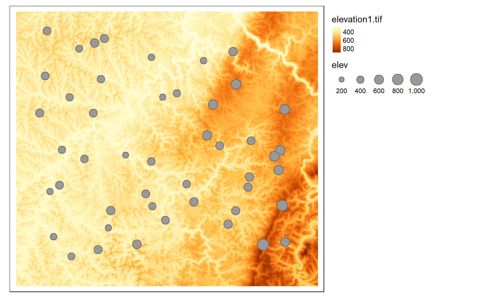
ws_mn_elev <- terra::extract(elev, ws2, fun=mean)
ws_mn_elev2 <- ws_mn_elev

ws$elev <- as.numeric(ws_mn_elev2$elevation1)

tm_shape(ws)+
  tm_polygons(col="elev")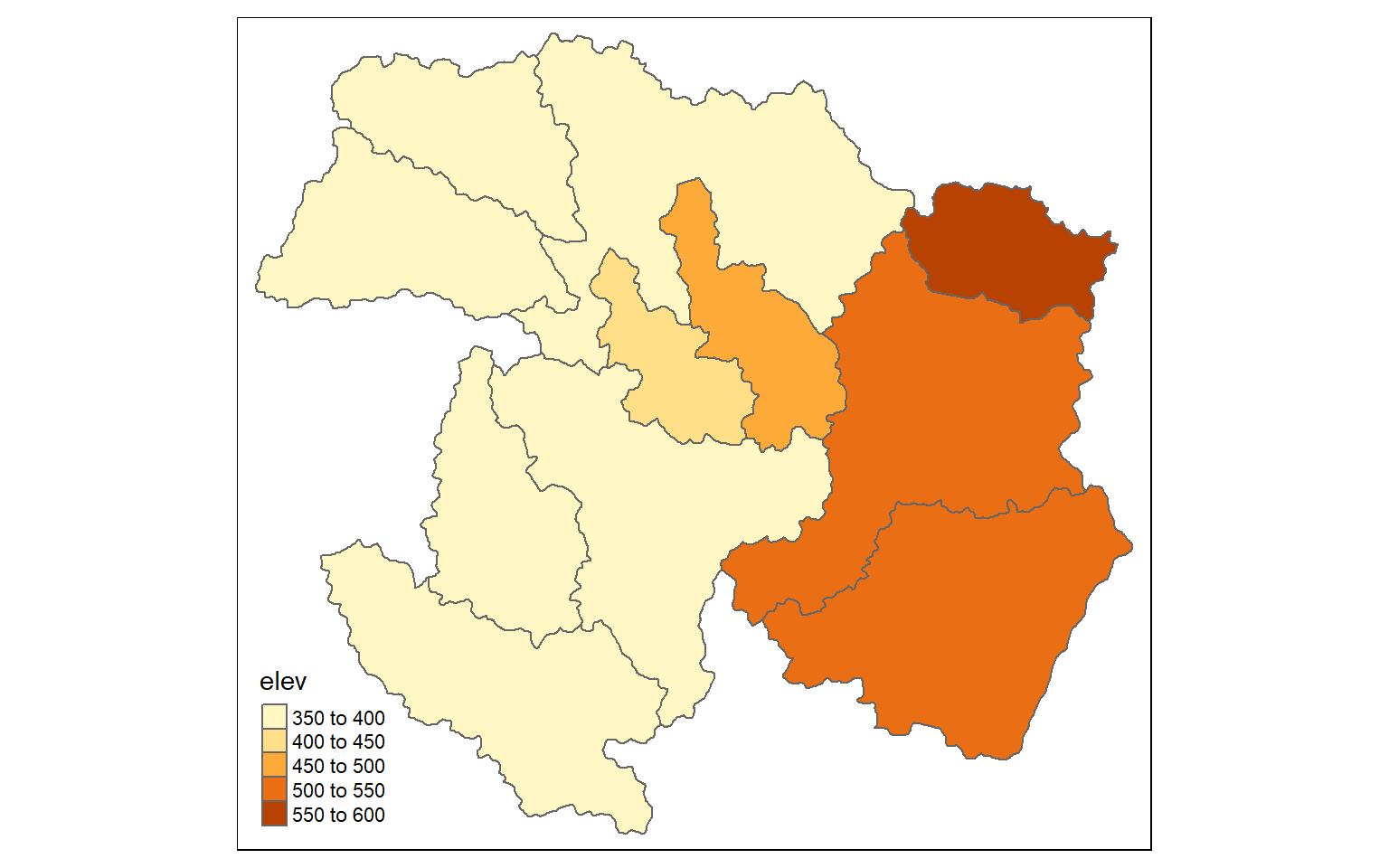
Raster Math
Mathematical and logical operations can be performed on raster data. Below, I have provided several examples. In the first example, I am finding all cell values in a land cover dataset that are classified as deciduous forest (41), evergreen forest (42), mixed forest (43), or woody wetland (90). Cells that return TRUE for the logic will be coded as 1 in the output while cells that return FALSE will be coded to zero. Thus, the result will be a binary raster.
forest <- lc ==41 | lc==42 |lc==43 | lc==90
tm_shape(forest)+
  tm_raster(style= "cat", labels = c("Not Forest", "Forest"), palette = c("gray", "darkolivegreen"))
In the next example, I multiply each cell by a constant to convert elevation in meters to elevation in feet. It is possible to perform mathematical operations (+, -, /, *) between each cell in a raster and a constant value or between overlapping cells in multiple raster grids. If multiple raster grids are used, they must have the same origin and extent.
dem_ft <- dem*3.28084

tm_shape(dem_ft)+
  tm_raster(style= "cont", palette=get_brewer_pal("-Greys", plot=FALSE))+
  tm_layout(legend.outside = TRUE)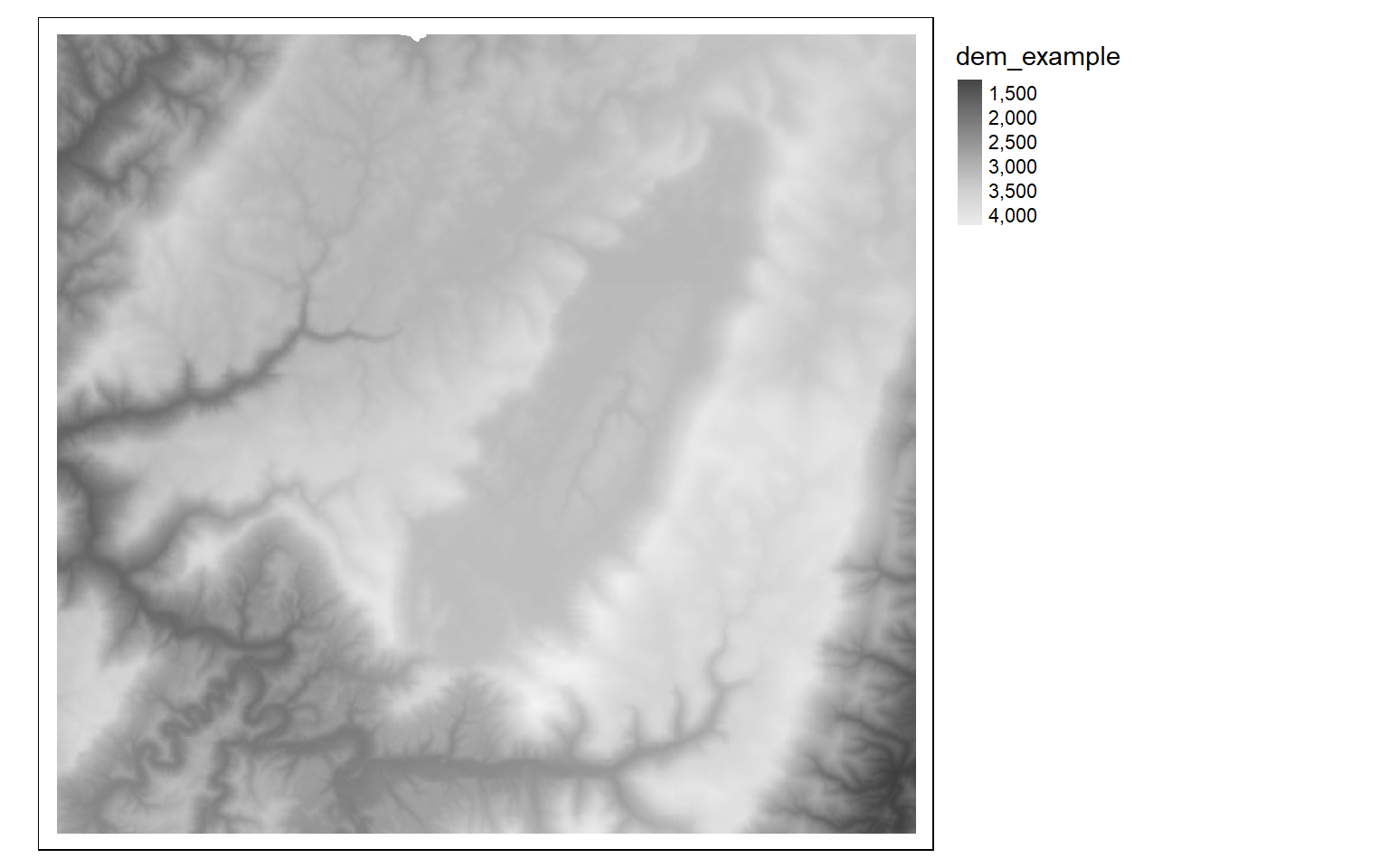
The example below includes logical statements applied to multiple grids. Specifically, cells will be coded to 1 in the output spatRaster if they are evergreen forest (42) OR mixed forest (43) AND are at an elevation greater than 1,000 meters. Note that I first need to align the two grids. To accomplish this, I use the resample() function to align the DEM to the land cover data. Again, terra is less forgiving to differences in origin and spatial extent than GIS software, such as ArcGIS Pro.
dem2 <- resample(dem, lc, "bilinear")
biOut <- (lc==42 | lc == 43) & (dem2 > 1000)

tm_shape(biOut)+
  tm_raster(style= "cat", labels = c("Not Suitable", "Suitable"), palette = c("gray", "salmon"))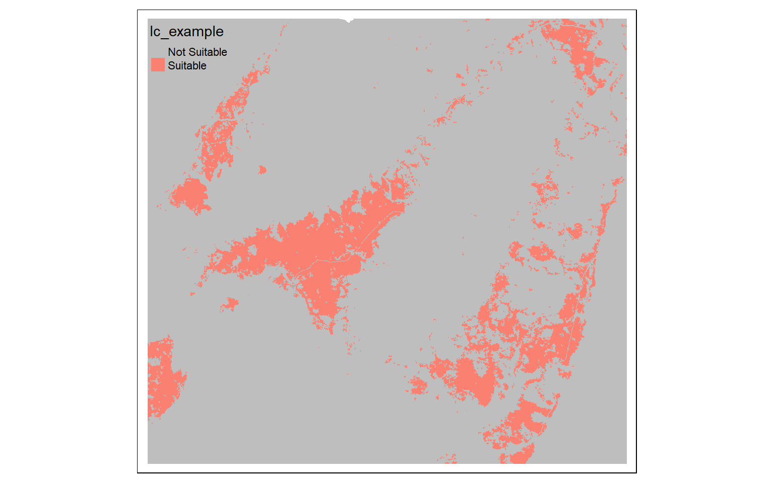
Distance Grids
The distance() function can be used to obtain a raster grid of distances from origin features relative to the map projection. The origin features can be points, lines, or polygon vector data; a table of x,y coordinates; or another spatRaster. If a raster grid is used, the distance will be calculated from the nearest cell that is not NULL or NA. In the examples below, I calculate the distance from point features representing airports and line features representing interstates. Each cell location in the spatial extent of the elev raster will be calculated; it is necessary to provide a reference grid used to define the origin, extent, cell size, and coordinate reference system of the resulting spatRaster object. There is also a costDistance() function that allows for the incorporation of a frictional, cost, or weighting surface. For example, you could calculate the distance form streams weighted by topographic slope. Note that these methods can be slow.
air <- vect("C:/terraWS/wv/airports.shp")
air2 <- st_read("C:/terraWS/wv/airports.shp")
Reading layer `airports' from data source `C:\terraWS\wv\airports.shp' using driver `ESRI Shapefile'
Simple feature collection with 101 features and 9 fields
Geometry type: POINT
Dimension:     XY
Bounding box:  xmin: 363896.7 ymin: 4123139 xmax: 765733.2 ymax: 4497709
Projected CRS: WGS 84 / UTM zone 17N

dist <- distance(elev, air)

|---------|---------|---------|---------|
=========================================


tm_shape(dist)+
  tm_raster(style= "cont")+
  tm_shape(air2)+
  tm_bubbles()+
  tm_layout(legend.outside=TRUE)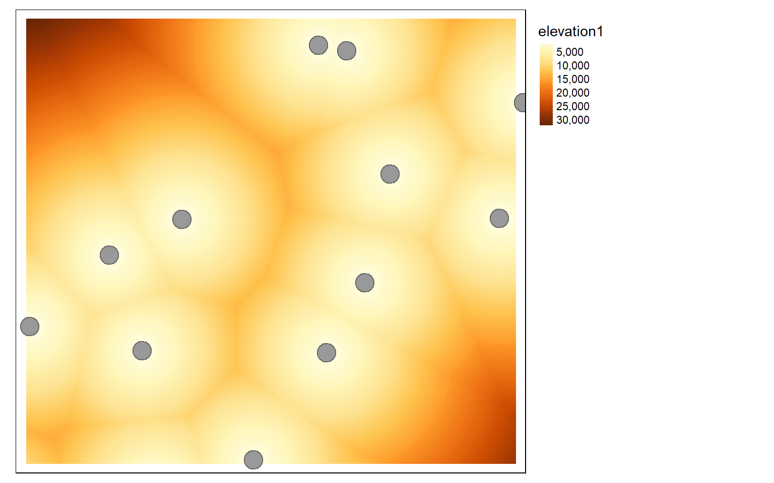
inter <- vect("C:/terraWS/wv/interstates.shp")
inter2 <- st_read("C:/terraWS/wv/interstates.shp")
Reading layer `interstates' from data source `C:\terraWS\wv\interstates.shp' using driver `ESRI Shapefile'
Simple feature collection with 47 features and 14 fields
Geometry type: LINESTRING
Dimension:     XY
Bounding box:  xmin: 360769.4 ymin: 4125421 xmax: 772219.7 ymax: 4438518
Projected CRS: WGS 84 / UTM zone 17N

dist2 <- distance(elev, inter)

|---------|---------|---------|---------|
=========================================


tm_shape(dist2)+
  tm_raster(style= "cont")+
  tm_shape(inter2)+
  tm_lines(col="black")+
  tm_layout(legend.outside=TRUE)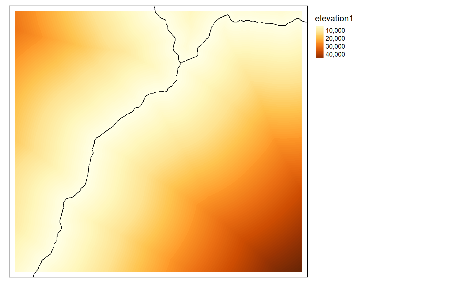
Image Analysis
In this section, we will explore some common image analysis tasked used in remote sensing.
Band Indices and Spectral Enhancements
Band indices can be calculated using raster math. Below I calculate the normalized difference vegetation index (NDVI) from the NIR and red bands followed by a normalized difference water index (NDWI) from the green and NIR bands. I also add a small number to the denominator to avoid a divide by zero error. In the final code block I use the c() function to add these derivatives as new layers or bands to the spatRaster created from the original Sentinel-2 MSI image.
Note also the use of the get_brewer_pal() function to define the color palette, which was discussed above. Again, this function is made available by the RColorBrewer package, which provides access to recommended color palettes that may be familiar to GIS and cartography professionals and are also available at this website.
s2ndvi <- (s2$nir-s2$red)/((s2$nir+s2$red)+.0001)
names(s2ndvi) <- "ndvi"

tm_shape(s2ndvi)+
  tm_raster(style= "cont", palette=get_brewer_pal("Greens", plot=FALSE))+
  tm_layout(legend.outside=TRUE)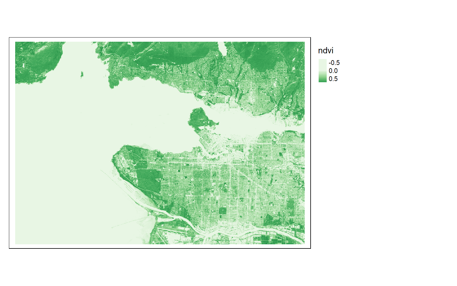
s2ndwi <- (s2$green-s2$nir)/((s2$green+s2$nir)+.0001)
names(s2ndwi) <- "ndwi"

tm_shape(s2ndwi)+
  tm_raster(style= "cont", palette=get_brewer_pal("Blues", plot=FALSE))+
  tm_layout(legend.outside=TRUE)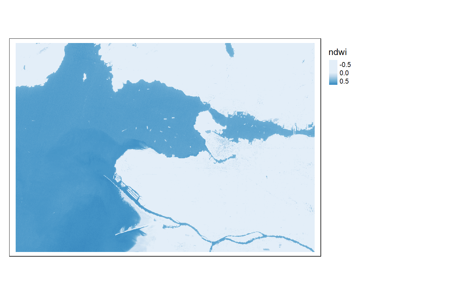
s2add <- c(s2, s2ndvi, s2ndwi)
names(s2add)
[1] "blue"  "green" "red"   "nir"   "swir1" "swir2" "ndvi"  "ndwi"
The following code blocks provide another example of implementing band indices. In this case, the difference normalized burn ratio (dNBR) is calculated from pre- and post-fire Landsat 7 ETM+ scenes for a fire that occurred in the Black Hills area of South Dakota. This workflow includes the following steps.
- Read in the images. Note that the data have already been converted to surface reflectance.
- Display the images as false color composites with plotRGB() using the SWIR2, NIR, and green bands. The extent of the fire is obvious in the post-fire image.
- Rename the image bands using name().
- Calculate the pre- and post-fire normalized burn ratio (NBR) from each image.
- Subtract the results to obtain the dNBR.
- Display the result.
- Reclassify the continuous dNBR result into “Not Burned”, “Low Severity”, “Moderate Severity”, and “High Severity” classes using classify().
- Display the classified result with a custom color mapping.
pre <- rast("C:/terraWS/blackhills/pre_ref2.img")
post <- rast("C:/terraWS/blackhills/post_ref2.img")

plotRGB(pre, r=6, g=4, b=2, stretch="lin")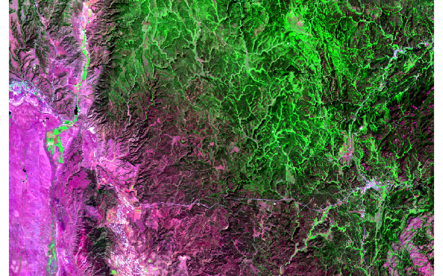
plotRGB(post, r=6, g=4, b=2, stretch="lin")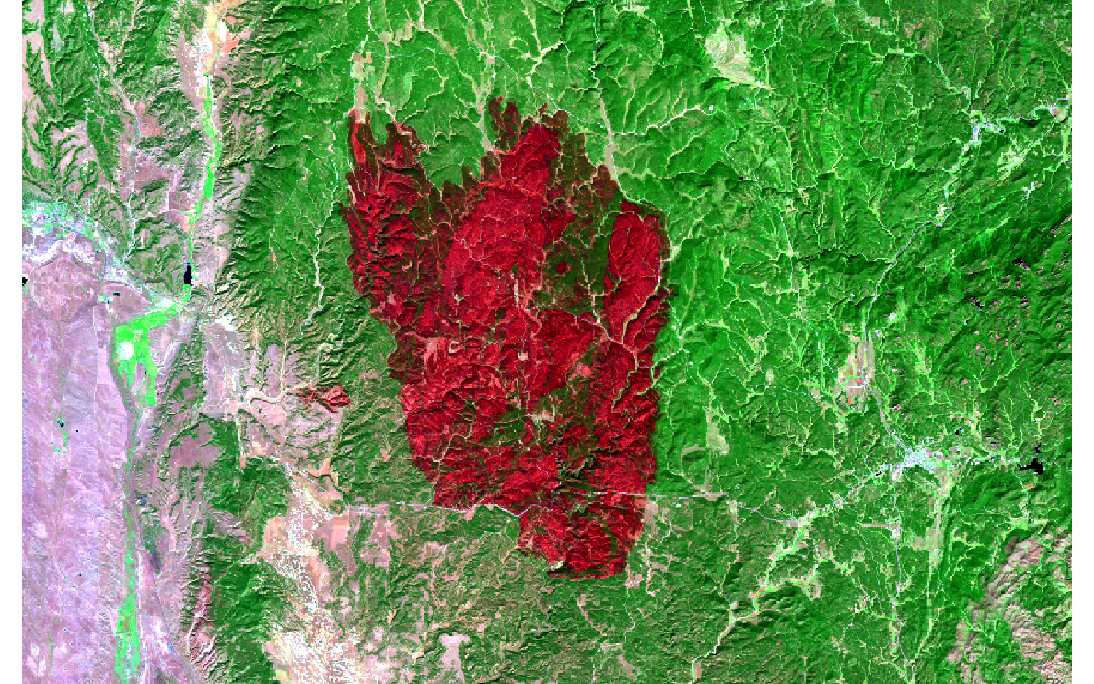
names(pre) <- c("Blue", "Green", "Red", "NIR", "SWIR1", "SWIR2")
names(post) <- c("Blue", "Green", "Red", "NIR", "SWIR1", "SWIR2")

pre_nbr <- (pre$NIR - pre$SWIR2)/((pre$NIR + pre$SWIR2)+.0001)

post_nbr <- (post$NIR - post$SWIR2)/((post$NIR + post$SWIR2)+.0001)

dnbr <- pre_nbr - post_nbr

tm_shape(dnbr)+
tm_raster(style= "equal", n=7, palette=get_brewer_pal("YlOrRd", n = 7, plot=FALSE))+
tm_layout(legend.outside = TRUE)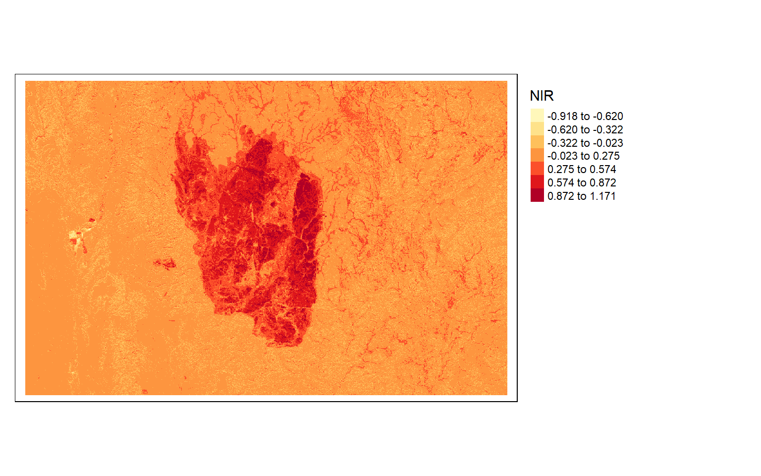
m <- c(-1000, .1, 0,  .1, .27, 1,  .27,
       .66,  2, .66, 1000, 3)
m <- matrix(m, ncol=3, byrow = TRUE)

dnbrCls <- classify(dnbr, m, right=TRUE)

tm_shape(dnbrCls)+
  tm_raster(style= "cat", labels = c("Not Burned", "Low Severity", "Medium Severity", "High Severity"), palette = c("gray", "yellow", "orange", "red"), title="Burn Severity")+
  tm_layout(legend.outside = TRUE)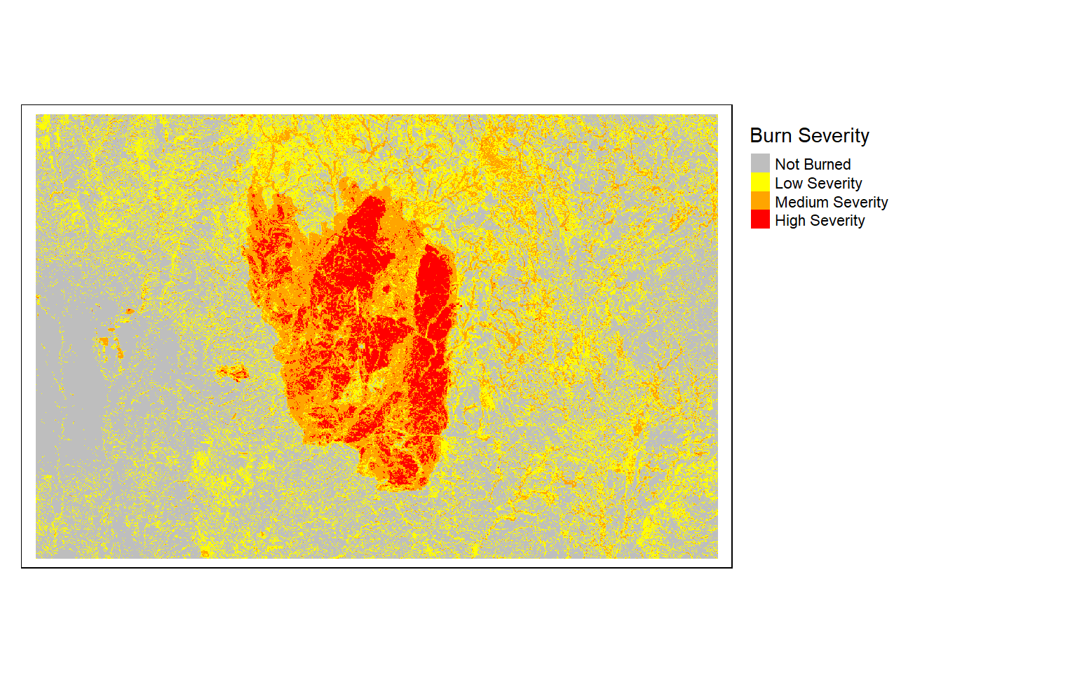
Principal Component Analysis, or PCA, can be performed on image data using the RStoolbox package. The rasterPCA() function can accept spatRaster objects as input. In the series of code blocks below I first perform the PCA to obtain the same number of components as the original number of bands in the image. Setting the spca argument to TRUE results in a standardized PCA in which all bands are centered and scaled.
Once the PCA is performed, I then write the resulting principal components to a new spatRaster object and display them with plotRGB(). The PCA object contains additional information for understanding the analysis, such as the variance in the original bands explained by each component and the loadings associated with each band to generate each principal component.
So, terra does not provide functions to perform PCA. However, the RStoolbox package can accept spatRaster objects. I recommended exploring other tools made available in this package.
s2PCA <- rasterPCA(s2, nSamples = NULL, nComp = nlyr(s2), spca = TRUE)s2PCAImg <- rast(s2PCA$map)
plotRGB(s2PCAImg, r=1, b=2, g=3, stretch="lin")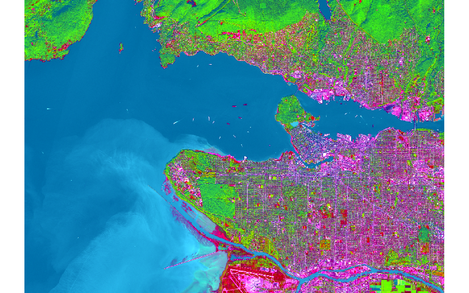
s2PCA$model
Call:
princomp(cor = spca, covmat = covMat[[1]])

Standard deviations:
    Comp.1     Comp.2     Comp.3     Comp.4     Comp.5     Comp.6
2.17044692 1.01096962 0.46407968 0.16944846 0.11552048 0.09835094

6 variables and 5879452 observations.s2PCA$model$loadings
Loadings:
Comp.1 Comp.2 Comp.3 Comp.4 Comp.5 Comp.6
blue 0.399 0.474 0.189 0.503 0.564
green 0.433 0.298 0.277 0.166 -0.770 -0.164
red 0.437 0.283 -0.823 0.150 0.169
nir 0.317 -0.655 0.636 0.181 -0.175
swir1 0.416 -0.384 -0.354 0.196 -0.148 0.703
swir2 0.434 -0.172 -0.597 0.109 -0.641
Comp.1 Comp.2 Comp.3 Comp.4 Comp.5 Comp.6
SS loadings 1.000 1.000 1.000 1.000 1.000 1.000
Proportion Var 0.167 0.167 0.167 0.167 0.167 0.167
Cumulative Var 0.167 0.333 0.500 0.667 0.833 1.000Focal Analysis and Convolution
Now that we have explored the generation of band indices and other spectral enhancements, we will move on to spatial enhancements. terra provides the focal() function, which allow for moving windows to be applied to images to perform convolutional operations, such as smoothing or edge detection. This process requires defining a filter or kernel as a two-dimensional matrix that is then passed over the image to perform the convolution.
In the first example, I am smoothing the NDVI result obtained above by passing a 5-by-5 cell kernel over the image where each cell has a weight of 1/25. So, all 25 cells in a window are multiplied by 1/25 then the results are added together to obtain the average in the window. The result is then returned to the center cell, and the window moves on to the next cell to process. This process continues until all cells have been processed or the moving window works across the entire grid.
ndvi5 <- focal(s2ndvi, w=matrix(1/25,nrow=5,ncol=5))

tm_shape(ndvi5)+
tm_raster(style= "quantile", n=7, palette=get_brewer_pal("Greens", n = 7, plot=FALSE))+
tm_layout(legend.outside = TRUE)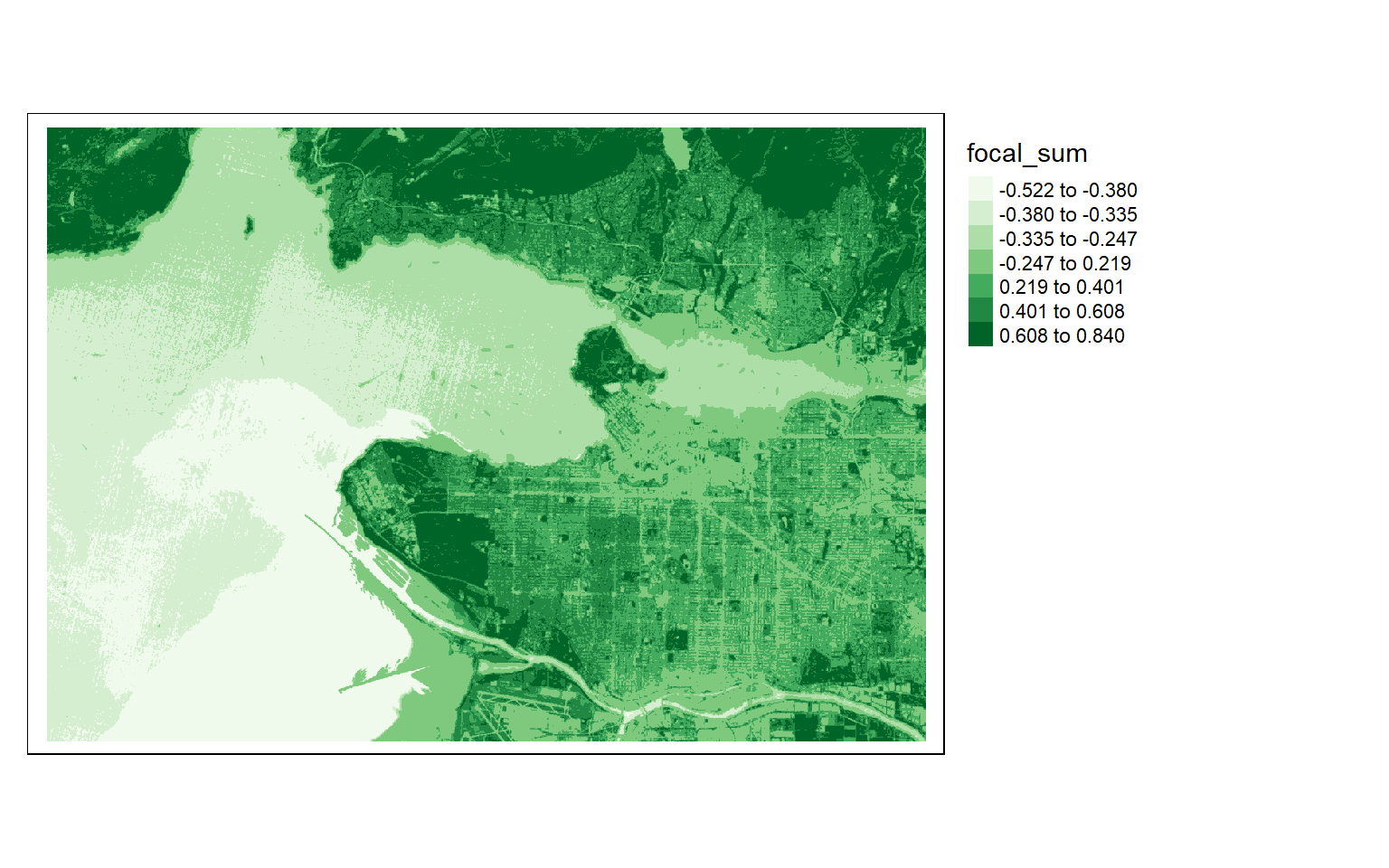
The Sobel filter is used to detect edges in images and raster data in general. It can be applied using different size kernels, such as 3-by-3 or 5-by-5. In the next code block, I am building then printing two 5-by-5 Sobel filters to detect edges in the x- and y-directions.
Once the filters are generated, I apply them to the NDVI data to detect edges, or changes in NDVI values. Mapping the results, we can see that these filters do indeed highlight edges.
There are many different filters that can be applied to images. Fortunately, the process is effectively the same once you build the required filter as a matrix.
gx <- c(2, 2, 4, 2, 2, 1, 1, 2, 1, 1, 0, 0, 0, 0, 0, -1, -1, -2, -1, -1, -1, -2, -4, -2, -2)
gy <- c(2, 1, 0, -1, -2, 2, 1, 0, -1, -2, 4, 2, 0, -2, -4, 2, 1, 0, -1, -2, 2, 1, 0, -1, -2, 2, 1, 0, -1, -2)

gx_m <- matrix(gx, nrow=5, ncol=5, byrow=TRUE)
gx_m
     [,1] [,2] [,3] [,4] [,5]
[1,]    2    2    4    2    2
[2,]    1    1    2    1    1
[3,]    0    0    0    0    0
[4,]   -1   -1   -2   -1   -1
[5,]   -1   -2   -4   -2   -2

gy_m <- matrix(gy, nrow=5, ncol=5, byrow=TRUE)
gy_m
     [,1] [,2] [,3] [,4] [,5]
[1,]    2    1    0   -1   -2
[2,]    2    1    0   -1   -2
[3,]    4    2    0   -2   -4
[4,]    2    1    0   -1   -2
[5,]    2    1    0   -1   -2
ndvi_edgex <- focal(s2ndvi, w=gx_m)
ndvi_edgey <- focal(s2ndvi, w=gy_m) tm_shape(ndvi_edgex)+
tm_raster(style= "quantile", n=7, palette=get_brewer_pal("-Greys", n = 7, plot=FALSE))+
tm_layout(legend.outside = TRUE)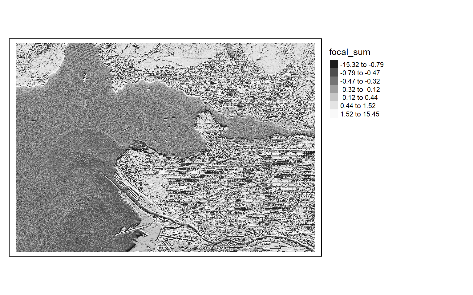
tm_shape(ndvi_edgey)+
tm_raster(style= "quantile", n=7, palette=get_brewer_pal("-Greys", n = 7, plot=FALSE))+
tm_layout(legend.outside = TRUE)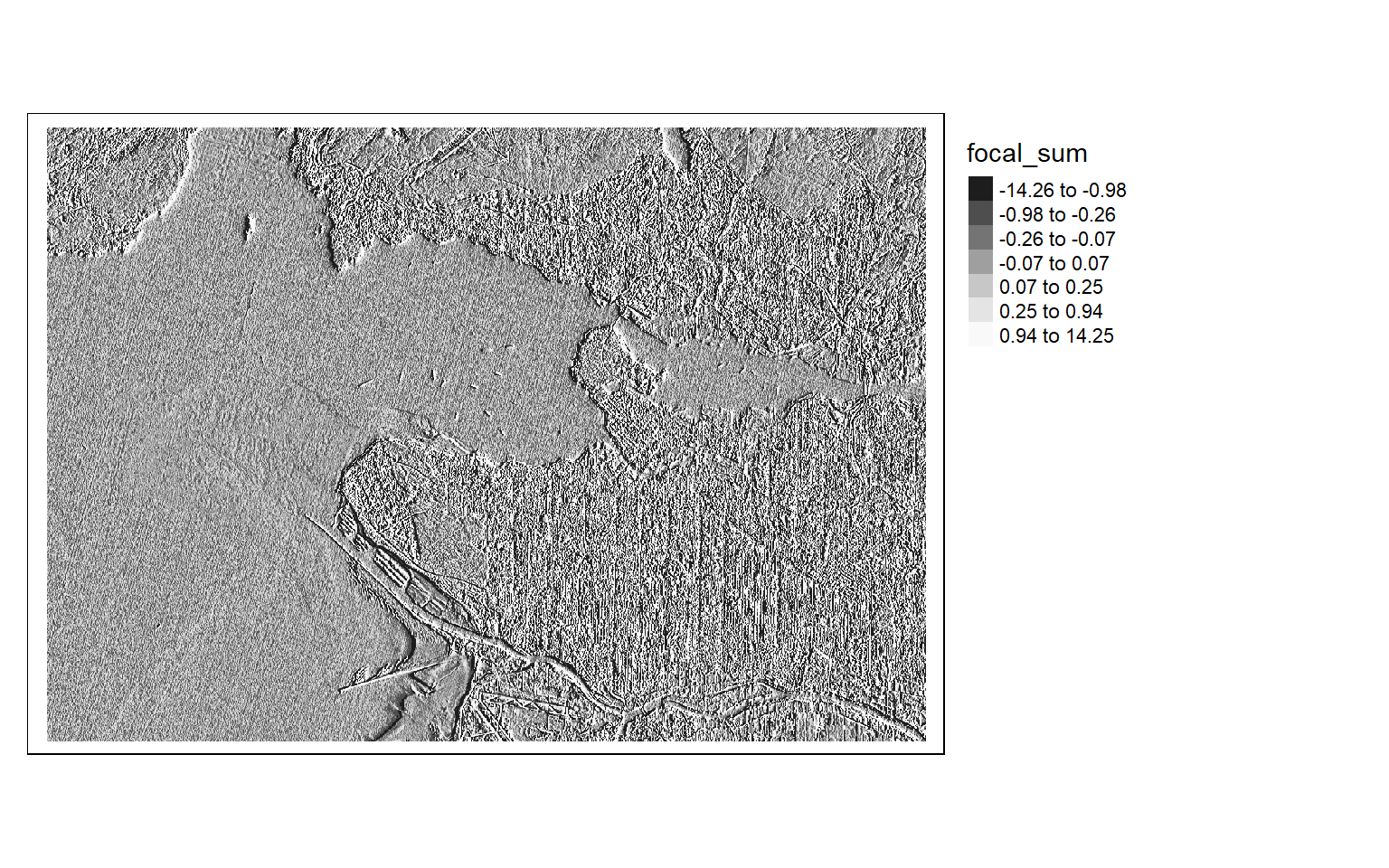
The focalMat() function allows for additional control and ability to define moving windows. With this function, you can define Gaussian, rectangular, and circular filters or kernels. When defining a circular filter, you can set cells within the square matrix that are outside of the circle to NA so that they are ignored in the calculations.
In the first example below, I apply a circular window to the NDVI data to obtain a smoothed representation of the result. To accomplish this, I first define a circular filter with a 90 meter radius. I then apply this to the NDVI data to obtain the mean within the circular moving window centered over each cell, effectively smoothing the original NDVI data. Within the focal() function, the fun argument can be used to specify what statistic to calculate within the moving window defined using focalMat().
myCircle <- focalMat(s2ndvi, 70, type="circle", fillNA=TRUE)

ndviCircle <- focal(s2ndvi, w=myCircle, fun=mean)

tm_shape(ndviCircle)+
tm_raster(style= "quantile", n=7, palette=get_brewer_pal("Greens", n = 7, plot=FALSE))+
tm_layout(legend.outside = TRUE)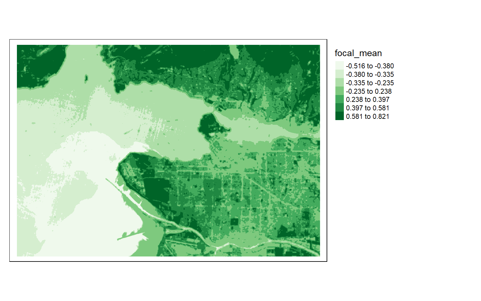
Moving window operations can also be useful for analyzing digital terrain data. In the code block below, I use a circular kernel to calculate the mean of elevation values. I then subtract this mean from the original digital elevation data to obtain a topographic position index, or TPI, in which high values indicate local topographic high points, such as ridges, and low values indicate local topographic low points, such as valleys.
dem <- rast("C:/terraWS/canaan/dem_example.tif")

myCircle <- focalMat(dem, 90, type="circle", fillNA=TRUE)

demMean <- focal(dem, w=myCircle, fun=mean)

tpi <- dem - demMean

tm_shape(tpi)+
tm_raster(style= "cont", palette=get_brewer_pal("-Greys", plot=FALSE))+
tm_layout(legend.outside = TRUE)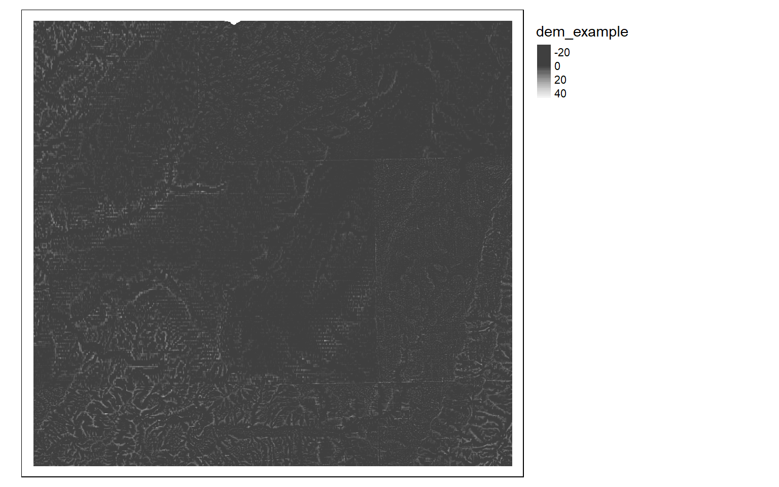
Although the analysis of digital elevation data was not a focus of this module, it is worth mentioning that terra does provide some useful functions for working with digital elevation data. For example, the terrain() function can be used to create a variety of terrain derivatives including slope, aspect, topographic position index (TPI), terrain ruggedness index (TRI), roughness, and flow direction. A hillshade can be generated with the shade() function and requires a slope and aspect surface as input, both of which should be in radian units. Some additional topographic metrics can be generated using the spatialEco package.
slp <- terrain(dem, "slope", unit="degrees", neighbors=8)

tm_shape(slp)+
tm_raster(style= "cont", palette=get_brewer_pal("-Greys", plot=FALSE))+
tm_layout(legend.outside = TRUE)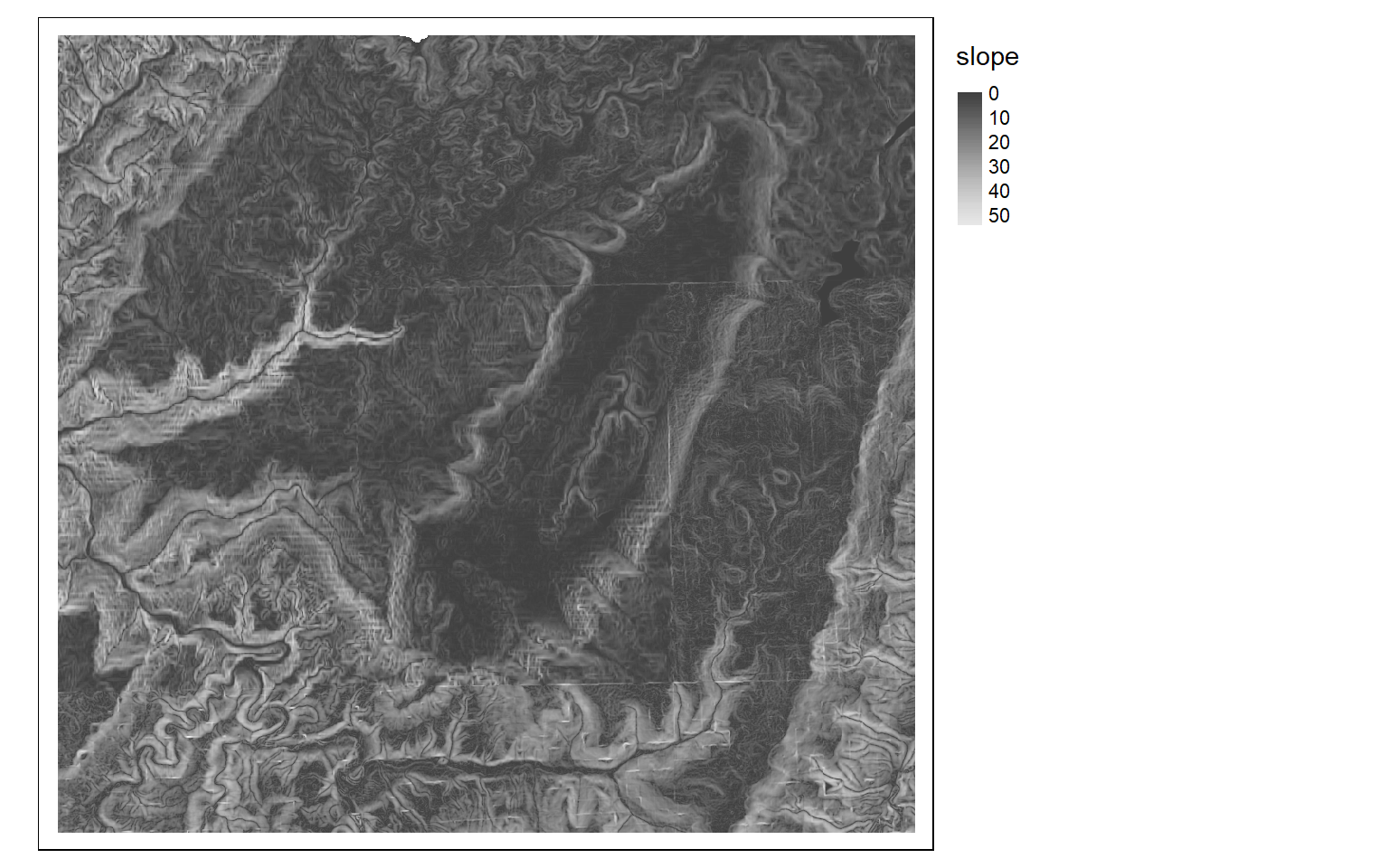
slp <- terrain(dem, "slope", unit="radians", neighbors=8)
asp <- terrain(dem, "aspect", unit="radians", neighbors=8)
hs <-  shade(slp, asp, angle=45, direction = 315, normalize=TRUE)

tm_shape(hs)+
tm_raster(style= "cont", palette=get_brewer_pal("-Greys", plot=FALSE))+
tm_layout(legend.outside = TRUE)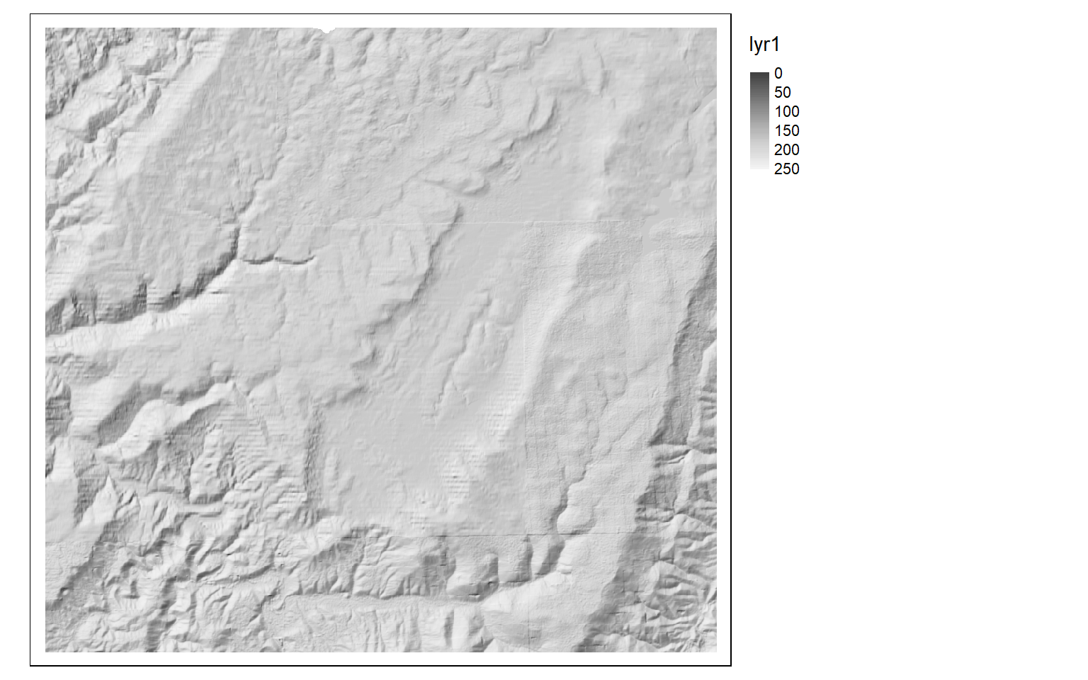
Supervised Classification
This final section will demonstrate how to perform a supervised classification using terra and machine learning algorithms implemented in R. First, we will read in some vector points representing training data and a Sentinel-2 MSI image of the area around Alexandria, Egypt collected on August 8, 2020. The image has a 10 m spatial resolution and contains 10 bands: blue, green, red, red edge 1, red edge 2, red edge 3, NIR, narrow NIR, SWIR1, and SWIR2. Bands that were collected at a coarser cell size were resampled to a 10-by-10 m cell size to match the higher spatial resolution data. I then change the band names so that they are more meaningful.
trainPts <- vect("C:/terraWS/alexandria/alexandria_points.shp")
alex <- rast("C:/terraWS/alexandria/s2_2020_08_04_alexandria.tif")

names(alex) <- c("blue", "green", "red", "RE1", "RE2", "RE3", "NIR", "NIRN", "SWIR1", "SWIR2")
alex
class       : SpatRaster
dimensions  : 10980, 10980, 10  (nrow, ncol, nlyr)
resolution  : 10, 10  (x, y)
extent      : 699960, 809760, 3390240, 3500040  (xmin, xmax, ymin, ymax)
coord. ref. : WGS_1984_UTM_Zone_35N (EPSG:32635)
source      : s2_2020_08_04_alexandria.tif
names       :  blue, green,   red,   RE1,   RE2,   RE3, ...
min values  :     1,     1,     1,     1,     0,     0, ...
max values  : 19728, 14784, 14472, 14896, 11650, 10467, ...
Next, I use dplyr to count the number of samples in each class. First, this requires converting the spatVector object to an sf object.
trainPts2 <- st_as_sf(trainPts)
trainPts2 %>% group_by(Classname) %>% count()
Simple feature collection with 4 features and 2 fields
Geometry type: MULTIPOINT
Dimension:     XY
Bounding box:  xmin: 700958.5 ymin: 3391294 xmax: 808331.6 ymax: 3497872
Projected CRS: WGS 84 / UTM zone 35N
# A tibble: 4 x 3
  Classname      n                                                      geometry
* <chr>      <int>                                              <MULTIPOINT [m]>
1 Developed    126 ((748499.2 3415504), (748716.7 3415739), (748956 3415569), (~
2 Sand/Rock     95 ((700958.5 3396986), (701174.3 3395625), (701539.4 3391875),~
3 Vegetation   229 ((755467.6 3411784), (755873.8 3411465), (756249.8 3411982),~
4 Water        104 ((704401.6 3447522), (707665.9 3475615), (708853 3497872), (~
Using terra and the extract() function, I then extract the band values at all of the sample locations. This results in a data frame. I then add the class name from the original point data to this data frame.
trainExt <- extract(alex, trainPts)
trainExt$class <- trainPts$Classname
In order to validate the result, I split the available samples into separate testing and training sets. Note that these samples are not randomized or correctly proportioned, so this is not a rigorous assessment. The sample_frac() function from dplyr allows for the extraction of random rows from a table. Setting the replace argument to FALSE results in random sampling without replacement. Combining this with group_by() allows for stratified random sampling by the class code. The set_diff() function is then used to separate out the rows or points not selected for training into a separate test set. Note that the machine learning algorithm that we will use will not accept data stored in a tibble, which is generated by dplyr. So, we must convert the training and testing tables into standard data frames.
train <- trainExt %>% group_by(class) %>% sample_frac(0.7, replace = FALSE)
test <- setdiff(trainExt, train)

train <- data.frame(train)
train$class <- as.factor(train$class)
test <- data.frame(test)
test$class <- as.factor(test$class)
I am now ready to train a model. In this example, I use the random forest algorithm as implemented in the randomForest package. Column 12 in the table represents the dependent variable or class code while columns 2 through 11 are the image bands. If you are interested in implementing machine learning in R, check out the caret package and tidymodels set of packages.
Once the model is trained, you can call it using the variable name to obtain some information about the results. Random forest also provides estimates of variable importance, which can be plotted with the varImpPlot() function. Note that these measures can be misleading if variables are correlated. For a more robust assessment of importance, see the permimp package.
mod1 <- randomForest(y=train[,12], x=train[,c(2:11)], importance=TRUE, ntree=10)
mod1

Call:
 randomForest(x = train[, c(2:11)], y = train[, 12], ntree = 10,      importance = TRUE)
               Type of random forest: classification
                     Number of trees: 10
No. of variables tried at each split: 3

        OOB estimate of  error rate: 0.26%
Confusion matrix:
           Developed Sand/Rock Vegetation Water class.error
Developed         87         0          0     0  0.00000000
Sand/Rock          1        64          0     0  0.01538462
Vegetation         0         0        159     0  0.00000000
Water 0 0 0 73 0.00000000varImpPlot(mod1)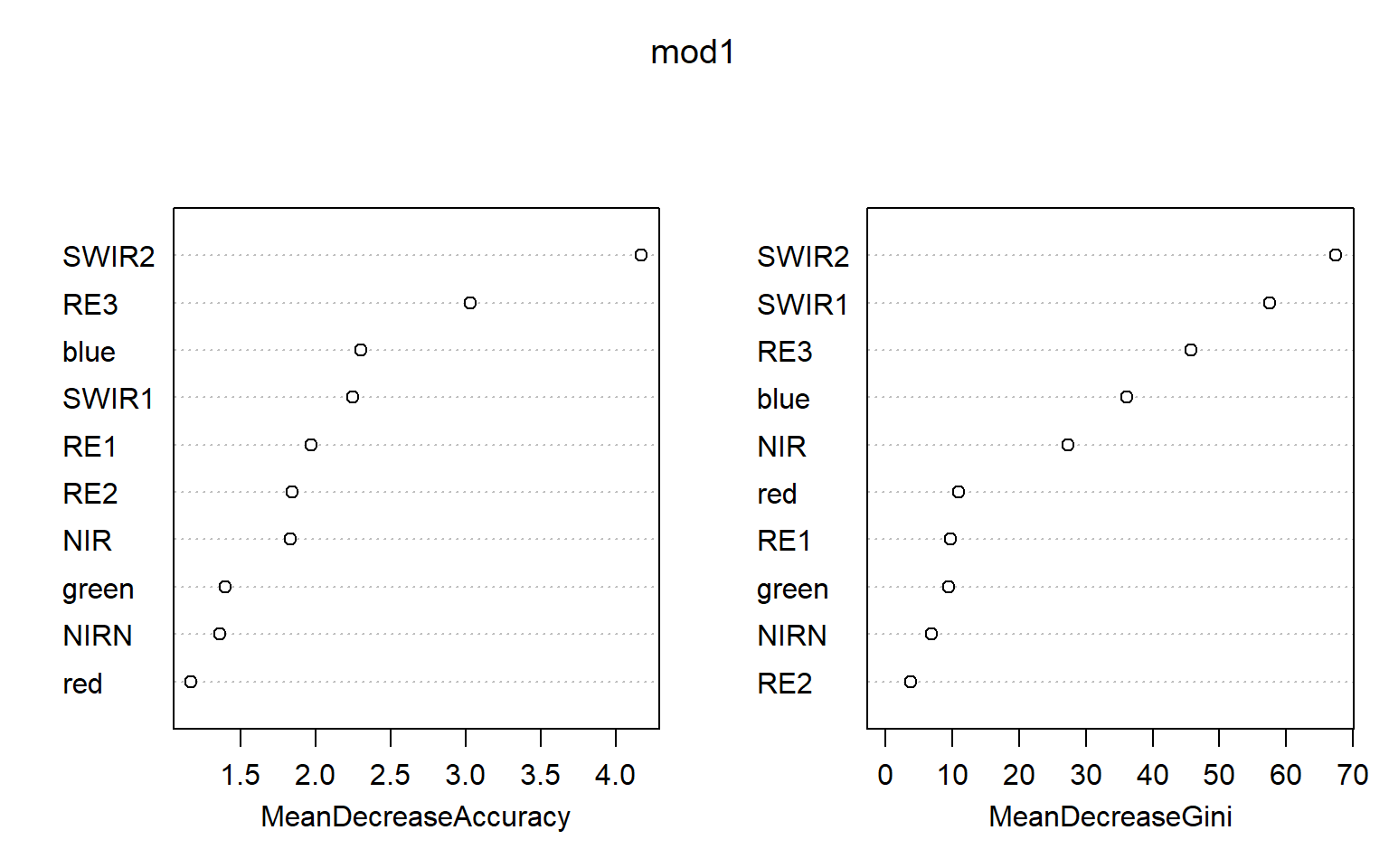
To assess the model using the withheld testing or validation samples, I first have to predict the data with the trained model using the predict() function. I then create a data frame that contains both the reference class and the predicted class. Next, I use the conf_mat() function from the yardstick package, which is part of tidymodels, to obtain a confusion matrix. Using the summary() function on the confusion matrix will provide a set of summary metrics.
In this case, we obtain nearly 100% accuracy. However, this is misleading as the samples were not randomly selected. In order to obtain informative assessment results, randomized validation data would need to be provided. However, the same methods and code could be applied.
pred <- predict(mod1, test)

forCF <- data.frame(ref=test$class, pred=pred)
conf_mat(forCF, ref, pred)
            Truth
Prediction   Developed Sand/Rock Vegetation Water
  Developed         35         0          0     0
  Sand/Rock          3        29          0     0
  Vegetation         0         0         69     0
  Water              0         0          0    31
summary(conf_mat(forCF, ref, pred))
# A tibble: 13 x 3
   .metric              .estimator .estimate
   <chr>                <chr>          <dbl>
 1 accuracy             multiclass     0.982
 2 kap                  multiclass     0.975
 3 sens                 macro          0.980
 4 spec                 macro          0.995
 5 ppv                  macro          0.977
 6 npv                  macro          0.994
 7 mcc                  multiclass     0.975
 8 j_index              macro          0.975
 9 bal_accuracy         macro          0.987
10 detection_prevalence macro          0.25
11 precision            macro          0.977
12 recall               macro          0.980
13 f_meas               macro          0.977
Predictions can be made back to raster data using the predict() function from terra. This requires that the same band names be applied so that the predictor variables can be mapped to the correct layers. In the example, I have read in a subset of the larger Alexandria Sentinel-2 image to predict to. Note that predicting to large images or datasets can be computationally and time intensive.
alex2 <- rast("C:/terraWS/alexandria/s2_2020_08_04_alexandria_sub.tif")
names(alex2) <- c("blue", "green", "red", "RE1", "RE2", "RE3", "NIR", "NIRN", "SWIR1", "SWIR2")
rastPred <- terra::predict(alex2, mod1)
Once the prediction is produced, I can then display it as a categorical raster using tmap.
tm_shape(rastPred)+
tm_raster(style= "cat",
labels = c("Developed", "Sand/Rock", "Vegetation", "Water"),
palette = c("salmon", "yellow", "green", "blue"),
title="Land Cover")+
tm_layout(legend.outside = TRUE)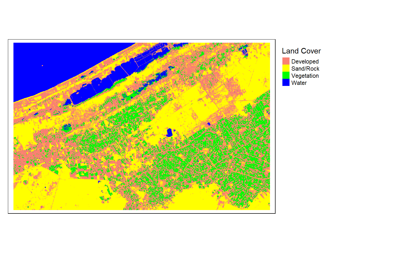
Conclusions and Final Remarks
Any spatRaster results generated with terra can be saved to disk using the writeRaster() function. I generally write to either TIFF or IMG format. Below is an example for saving the results of the supervised classification process.
writeRaster(rastPred, "C:/terraWS/alex_pred.tif", overwrite=TRUE)This is the end of this module. I hope you found it useful. If you would like to learn more about terra, please check out:
Visit this link for a more complete list of geospatial packages available in R.