Machine Learning with caret
Objectives
- Train models, predict to new data, and assess model performance using different machine learning methods and the caret package
- Define training controls to optimize models and tune hyperparameters
- Explore means to improve model performance using training data balancing, feature selection, and pre-processing
- Make categorical and continuous predictions
- Plot decision trees
Overview
Expanding upon the last section, we will continue exploring machine learning in R. Specifically, we will use the caret (Classification and Regression Training) package. Many packages provide access to machine learning methods, and caret offers a standardized means to use a variety of algorithms from different packages. This link provides a list of all models that can be used through caret. In this module, we will specifically focus on k-nearest neighbor (k-NN), decision trees (DT), random forests (RF), and support vector machines (SVM); however, after learning to apply these methods you will be able to apply many more methods using similar syntax. We will explore caret using a variety of examples. The link at the bottom of the page provides the example data and R Markdown file used to generate this module.
A cheat sheet for caret can be found here.
Before beginning, you will need to load in the required packages.
library(caret)
library(rpart.plot)
library(randomForest)
library(plyr)
library(dplyr)
library(raster)
library(sf)
library(rgdal)
library(tmap)
library(tmaptools)
library(Metrics)
library(forcats)
Example 1: Wetland Classification
In this first example, we will predict wetland categories using different algorithms and compare the results. The training variables were derived from Landsat imagery and include brightness, greenness, wetness, and NDVI from September and April imagery. Also, terrain variables were included to offer additional predictors. Four classes are differentiated: not wetlands (Not), palustrine emergent wetlands (PEM), palustrine forested wetlands (PFO), and rivers/lakes/ponds (RLP). These data have not been published or used in a paper.
First, I read in the data. Next, I subset 200 examples of each class for training (train) using functions from dplyr. Optimally, more samples would be used to train the models; however, I am trying to minimize training and tuning time since this is just a demonstration. I then use the setdiff() function to extract all examples that were not included in the training set to a validation set (val).
wetdata <- read.csv("caret/wetland_data2.csv", header=TRUE, sep=",", stringsAsFactors=TRUE)set.seed(42)
train <- wetdata %>% dplyr::group_by(class) %>% dplyr::sample_n(200, replace=FALSE)
val <- setdiff(wetdata, train)Now that I have created separate training and validation data sets, I can tune hyperparameters for the different models. Using the trainControl() function, I define the training and tuning parameters. Here, I am using cross validation with 5 folds. The available methods include:
- “boot”: bootstrap
- “cv”: k-fold cross validation
- “LOOCV”: leave-one-out cross validation
- “repeated”: repeated k-fold cross validation
I tend to use k-fold cross validation, bootstrapping, or repeated k-fold cross validation. The number argument for k-fold cross validation specifies the number of folds while it will determine the number of bootstrap samples for bootstrapping. A repeat argument is required for repeated k-fold cross validation. In the example, I am using 5-fold cross validation without repeats. I have also set the verboseIter argument to FALSE so that the results of each fold are not printed to the console. If you would like to monitor the progression of the hyperparameter tuning process, you can set this to TRUE. Optimally, I would use more folds and a larger training set; however, I am trying to speed up the process so that it doesn’t take very long to tune the algorithms. I generally prefer to use 10 folds. I am also setting a random seed to obtain consistent results and make the experiment more reproducible.
set.seed(42)
trainctrl <- trainControl(method = "cv", number = 5, verboseIter = FALSE)
In the next code block I am optimizing and training the four different models. Notice that the syntax is very similar. I only need to change the method to a different algorithm. I can also provide arguments specific to the algorithm; for example, I am providing an ntree argument for random forest. I am also centering and scaling the data for each model and setting the tuneLength to 10. So, ten values for each hyperparameter will be assessed using 5-fold cross validation. To fine tune a model, you should use a larger tune length; however, that will increase the time required. You can also provide your own list of values and implement tuneGrid as opposed to tuneLength. I am optimizing using the Kappa statistic, so the model with the best Kappa value will be returned as the final model. It is also possible to use overall accuracy as opposed to Kappa. Before running each model, I have set a random seed for reproducibility,
Note that it will take some time to tune and train these models if you choose to execute the code. Also, feel free to try different models. For example, the ranger package provides a faster implementation of random forest.
#Run models using caret
set.seed(42)
knn.model <- train(class~., data=train, method = "knn",
tuneLength = 10,
preProcess = c("center", "scale"),
trControl = trainctrl,
metric="Kappa")

set.seed(42)
dt.model <- train(class~., data=train, method = "rpart",
tuneLength = 10,
preProcess = c("center", "scale"),
trControl = trainctrl,
metric="Kappa")

set.seed(42)
rf.model <- train(class~., data=train, method = "rf",
tuneLength = 10,
ntree=100,
importance=TRUE,
preProcess = c("center", "scale"),
trControl = trainctrl,
metric="Kappa")

set.seed(42)
svm.model <- train(class~., data=train, method = "svmRadial",
tuneLength = 10,
preProcess = c("center", "scale"),
trControl = trainctrl,
metric="Kappa")
Once models have been trained and tuned, they can be used to predict to new data. In the next code block, I am predicting to the validation data. Note that the same predictor variables must be provided and they must have the same names. It is okay to include variables that are not used. It is also fine if the variables are in a different order.
Once a prediction has been made, I use the confusionMatrix() function to obtain assessment metrics. Based on the reported metrics, RF and SVM outperform the k-NN and DT algorithms for this specific task.
knn.predict <-predict(knn.model, val)
dt.predict <-predict(dt.model, val)
rf.predict <-predict(rf.model, val)
svm.predict <-predict(svm.model, val)confusionMatrix(knn.predict, val$class)
Confusion Matrix and Statistics
Reference
Prediction Not PEM PFO RLP
Not 1505 18 24 47
PEM 147 1240 282 119
PFO 123 490 1417 324
RLP 25 52 77 1310
Overall Statistics
Accuracy : 0.76
95% CI : (0.75, 0.7698)
No Information Rate : 0.25
P-Value [Acc > NIR] : < 2.2e-16
Kappa : 0.68
Mcnemar's Test P-Value : < 2.2e-16
Statistics by Class:
Class: Not Class: PEM Class: PFO Class: RLP
Sensitivity 0.8361 0.6889 0.7872 0.7278
Specificity 0.9835 0.8985 0.8265 0.9715
Pos Pred Value 0.9442 0.6935 0.6020 0.8948
Neg Pred Value 0.9474 0.8965 0.9210 0.9146
Prevalence 0.2500 0.2500 0.2500 0.2500
Detection Rate 0.2090 0.1722 0.1968 0.1819
Detection Prevalence 0.2214 0.2483 0.3269 0.2033
Balanced Accuracy 0.9098 0.7937 0.8069 0.8496confusionMatrix(dt.predict, val$class)
Confusion Matrix and Statistics
Reference
Prediction Not PEM PFO RLP
Not 1531 79 122 170
PEM 107 1332 472 118
PFO 139 336 1150 358
RLP 23 53 56 1154
Overall Statistics
Accuracy : 0.7176
95% CI : (0.7071, 0.728)
No Information Rate : 0.25
P-Value [Acc > NIR] : < 2.2e-16
Kappa : 0.6235
Mcnemar's Test P-Value : < 2.2e-16
Statistics by Class:
Class: Not Class: PEM Class: PFO Class: RLP
Sensitivity 0.8506 0.7400 0.6389 0.6411
Specificity 0.9313 0.8709 0.8457 0.9756
Pos Pred Value 0.8049 0.6565 0.5799 0.8974
Neg Pred Value 0.9492 0.9095 0.8754 0.8908
Prevalence 0.2500 0.2500 0.2500 0.2500
Detection Rate 0.2126 0.1850 0.1597 0.1603
Detection Prevalence 0.2642 0.2818 0.2754 0.1786
Balanced Accuracy 0.8909 0.8055 0.7423 0.8083confusionMatrix(rf.predict, val$class)
Confusion Matrix and Statistics
Reference
Prediction Not PEM PFO RLP
Not 1589 30 57 74
PEM 104 1321 324 137
PFO 58 353 1277 188
RLP 49 96 142 1401
Overall Statistics
Accuracy : 0.7761
95% CI : (0.7663, 0.7857)
No Information Rate : 0.25
P-Value [Acc > NIR] : < 2.2e-16
Kappa : 0.7015
Mcnemar's Test P-Value : 3.06e-11
Statistics by Class:
Class: Not Class: PEM Class: PFO Class: RLP
Sensitivity 0.8828 0.7339 0.7094 0.7783
Specificity 0.9702 0.8954 0.8891 0.9469
Pos Pred Value 0.9080 0.7004 0.6807 0.8300
Neg Pred Value 0.9613 0.9099 0.9018 0.9276
Prevalence 0.2500 0.2500 0.2500 0.2500
Detection Rate 0.2207 0.1835 0.1774 0.1946
Detection Prevalence 0.2431 0.2619 0.2606 0.2344
Balanced Accuracy 0.9265 0.8146 0.7993 0.8626confusionMatrix(svm.predict, val$class)
Confusion Matrix and Statistics
Reference
Prediction Not PEM PFO RLP
Not 1553 48 35 70
PEM 102 1277 305 107
PFO 61 389 1332 182
RLP 84 86 128 1441
Overall Statistics
Accuracy : 0.7782
95% CI : (0.7684, 0.7877)
No Information Rate : 0.25
P-Value [Acc > NIR] : < 2.2e-16
Kappa : 0.7043
Mcnemar's Test P-Value : 5.62e-09
Statistics by Class:
Class: Not Class: PEM Class: PFO Class: RLP
Sensitivity 0.8628 0.7094 0.7400 0.8006
Specificity 0.9717 0.9048 0.8830 0.9448
Pos Pred Value 0.9103 0.7130 0.6782 0.8286
Neg Pred Value 0.9550 0.9033 0.9106 0.9343
Prevalence 0.2500 0.2500 0.2500 0.2500
Detection Rate 0.2157 0.1774 0.1850 0.2001
Detection Prevalence 0.2369 0.2487 0.2728 0.2415
Balanced Accuracy 0.9172 0.8071 0.8115 0.8727As discussed and demonstrated in the prior module, random forest provides an assessment of variable importance. To obtain these measures after a model has been generated with caret, you will need to extract the final model to a new object then call the importance() function on it. By calling the model, we can see the OOB error rate and confusion matrix for the OOB data. Based on the OOB mean decrease in accuracy measure, topographic slope was the most important variable in the prediction. Generally, both spectral and topographic variables were important in the model. The OOB error rate was 24.6%, suggesting that roughly a quarter of the OOB data are misclassified on average. So, the performance isn’t great. However, this is a complex classification problem.
#Variable Importance RF/OOB Error RF
rf.model.final <- rf.model$finalModel
importance(rf.model.final)
                 Not        PEM       PFO       RLP MeanDecreaseAccuracy
a_ndvi2   5.74239672  5.9778701 12.601644 4.2124869            10.000872
abright   6.91729515 11.2023308  6.982464 6.0847881            12.608724
agreen    7.63587685  3.9760913  9.102786 7.6173366            11.053074
awet      6.98487614  6.0177666  5.054557 5.6133191            10.544203
s_ndvi    7.39448139  8.5656727  7.876298 0.9542089            14.124229
sbright   4.64701968 14.2204087  8.877035 5.0004584            17.358782
sgreen    5.94762932  3.5785531  6.669556 2.7279847             7.936331
swet      3.47939860  7.5277984  3.945337 2.2430319            10.207702
slp_d    16.62502681  6.4341151 12.345918 5.4415807            21.971194
diss_a   14.50122296  7.3490750  5.654878 2.7092294            15.785692
rough_a  10.10283171  7.5752717  8.527104 1.7674813            13.711659
sp_a      7.47914088  9.3065409  6.710554 5.0555033            12.303625
ctmi      3.69423817  1.6336448  3.511083 3.6621277             6.390287
curv_arc -0.91201199 -0.2576315  1.762561 4.1165854             3.547979
curv_pro  0.05324813  0.5897456  3.305928 3.8294161             4.235983
crv_pln   1.32975100 -1.7227436  2.445788 3.3088655             3.100601
         MeanDecreaseGini
a_ndvi2          45.81355
abright          53.87912
agreen           60.70916
awet             27.55160
s_ndvi           35.81947
sbright          57.90330
sgreen           27.05002
swet             30.14842
slp_d            79.31722
diss_a           44.55795
rough_a          40.15968
sp_a             38.32568
ctmi             16.41397
curv_arc         13.38326
curv_pro         15.16093
crv_pln          12.93003
rf.model.final

Call:
 randomForest(x = x, y = y, ntree = 100, mtry = min(param$mtry,      ncol(x)), importance = TRUE)
               Type of random forest: classification
                     Number of trees: 100
No. of variables tried at each split: 5

        OOB estimate of  error rate: 22.5%
Confusion matrix:
    Not PEM PFO RLP class.error
Not 174   9  15   2       0.130
PEM   6 153  32   9       0.235
PFO   6  44 137  13       0.315
RLP  10  13  21 156       0.220
The structure of the decision tree can be plotted using the plot() function. The rpart.plot package includes the prp() function which provides a prettier decision tree visualization. This also gives us a sense of what variables are most important in the model.
#Make better tree plot
dt.model.final <- dt.model$finalModel
plot(dt.model.final)
text(dt.model.final)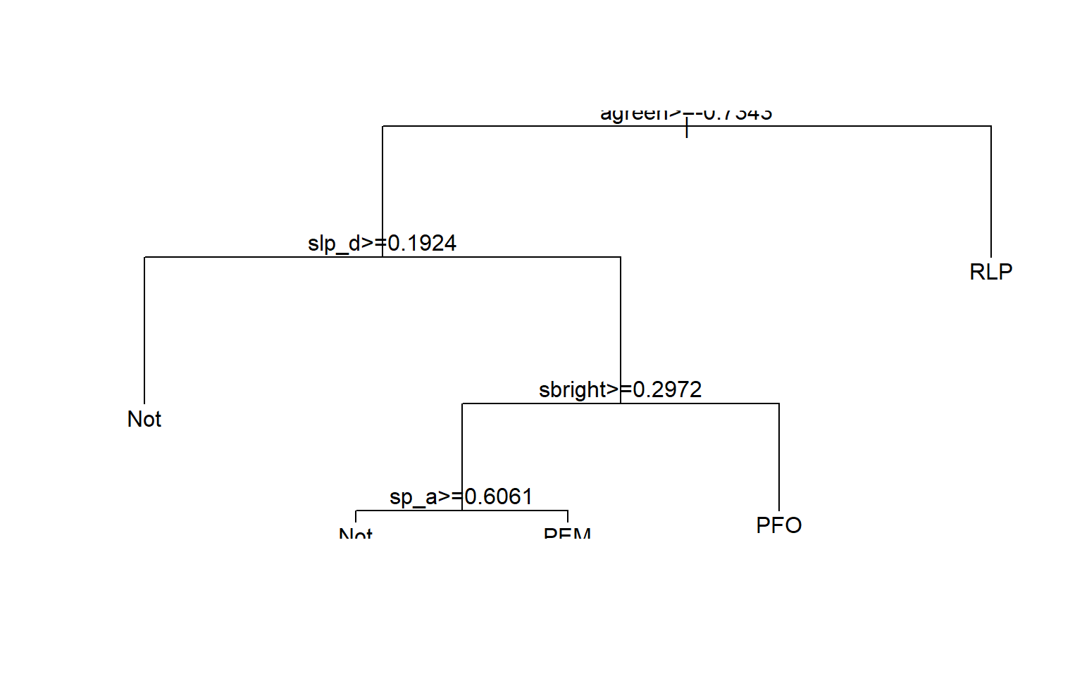
prp(dt.model.final)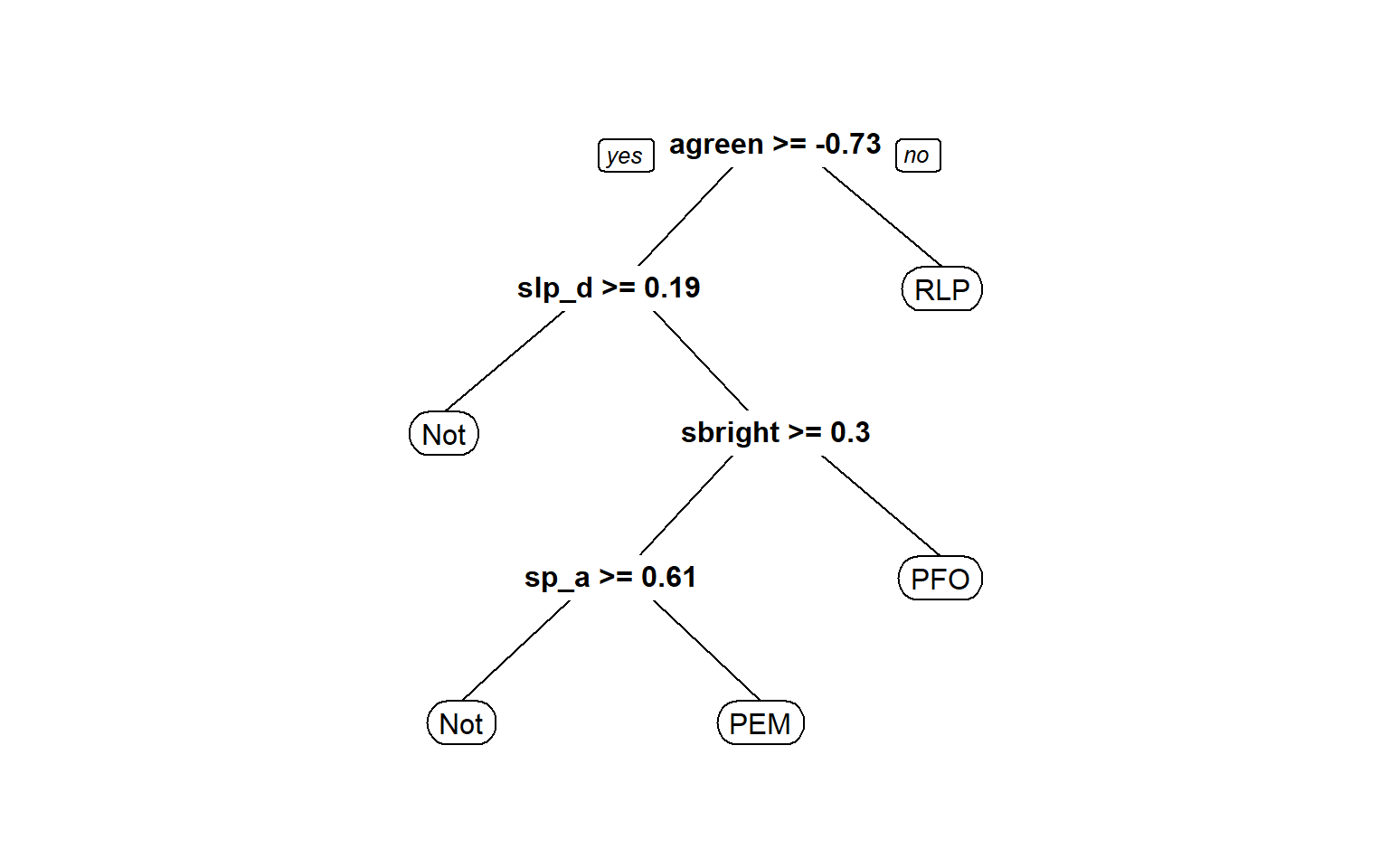
Example 2: Indian Pines
In this second example, I will demonstrate predicting crop types from hyperspectral imagery. The hyperspectral data are from the Airborne Visible/Infrared Imaging Spectrometer (AVIRIS), which offers 220 spectral bands in the visible, NIR, and SWIR spectrum. The following classes are differentiated:
- Alfalfa (54 pixels)
- Corn (2502 pixels)
- Grass/Pasture (523 pixels)
- Trees (1294 pixels)
- Hay (489 pixels)
- Oats (20 pixels)
- Soybeans (4050 pixels)
- Wheat (212 pixels)
These data are publicly available and cover the Indian Pines test site in Indiana. They can be obtained here. I have provided a raster representing the different categories (92av3gr8class.img), an image containing all the spectral bands (92av3c.img), and a mask to differentiate mapped and unmapped pixels (mask_ip.img).
Note that this example takes some time to execute, so you may choose to simply read through it as opposed to execute all the code.
classes <- raster("caret/92av3gr8class.img")
image <- stack("caret/92av3c.img")
mask <- raster("caret/mask_ip.img")head(classes@data@attributes, n=8)
[[1]]
ID COUNT Red Green Blue Class_Names Opacity
1 0 0 255 255 255 0
2 1 54 255 255 138 Alfalfa 255
3 2 2502 2 28 243 Corn 255
4 3 523 255 89 0 Grass/pasture 255
5 4 1294 5 255 133 Trees 255
6 5 489 255 2 250 Hay 255
7 6 20 89 0 255 Oats 255
8 7 4050 2 171 255 Soybeans 255
9 8 212 12 255 7 Wheat 255
I did not provide the training and validation data as tables in this example, so I will need to create them in R. To produce these data, I will use the process outlined below.
- Convert the classes grid to points
- Change the column names
- Remove all zero values since these represent pixels without a mapped class at that location
- Convert the “Class” field to a factor
- Change the “Class” field values from numeric codes to factors to improve interpretability
p <- st_as_sf(rasterToPoints(classes, fun=NULL, spatial=TRUE))
names(p) <- c("Class", "geometry")
p2 <- filter(p, Class > 0)
p2$Class <- as.factor(p2$Class)

p2$Class <- revalue(p2$Class, c("1"="Alfalfa", "2"="Corn", "3"="Grass/Pasture", "4"="Trees", "5"="Hay", "6"="Oats", "7"="Soybeans", "8"="Wheat"))- Next, I need to extract all the image bands at each mapped point or pixel location. This can be accomplished using the extract() function from the raster package. I then merge the resulting tables and remove the geometry field that is no longer required. Note that this can take some time since there are 220 bands to extract at each point location.
p3 <- as.data.frame(extract(image, p2))

data <- bind_cols(p2, p3)

st_geometry(data) <- NULL- Now that I have extracted the predictor variables at each mapped point, I will split the data into training (train) and testing (test) sets using dplyr. I divide the data such that 50% of the samples from each class will be used for training and the remaining half will be used for testing. I now have separate and non-overlapping test and training sets.
set.seed(42)
train <- data %>% group_by(Class) %>% sample_frac(0.5, replace=FALSE)

test <- setdiff(data, train)
I can now create models. First, I define the training and tuning controls to use 5-fold cross validation. I then tune and train each of the four models. I have set the tuneLength to 5, so only five values for each hyperparameter are tested. I am doing this to speed up the processes for demonstration purposes. However, if I were doing this for research purposes, I would test more values or use tuneGrid instead.
Again, if you choose to execute this code, it will take some time.
set.seed(42)
trainctrl <- trainControl(method = "cv", number = 5, verboseIter = FALSE)set.seed(42)
knn.model <- train(Class~., data=train, method = "knn",
tuneLength = 5,
preProcess = c("center", "scale"),
trControl = trainctrl,
metric="Kappa")
set.seed(42)
dt.model <- train(Class~., data=train, method = "rpart",
tuneLength = 5,
preProcess = c("center", "scale"),
trControl = trainctrl,
metric="Kappa")
set.seed(42)
rf.model <- train(Class~., data=train, method = "rf",
tuneLength = 5,
ntree = 100,
preProcess = c("center", "scale"),
trControl = trainctrl,
metric="Kappa")
set.seed(42)
svm.model <- train(Class~., data=train, method = "svmRadial",
tuneLength = 5,
preProcess = c("center", "scale"),
trControl = trainctrl,
metric="Kappa")Once the models are obtained, I predict to the withheld test data then created confusion matrices and accuracy assessment metrics. Take some time to review the confusion matrices to compare the models and assess what classes were most confused. Note that I provided an imbalanced training data set since there were different proportions of each class on the landscape.
knn.predict <-predict(knn.model, test)
dt.predict <-predict(dt.model, test)
rf.predict <- predict(rf.model, test)
svm.predict <-predict(svm.model, test)confusionMatrix(knn.predict, test$Class)
Confusion Matrix and Statistics
Reference
Prediction Alfalfa Corn Grass/Pasture Trees Hay Oats Soybeans Wheat
Alfalfa 2 0 0 0 1 0 0 0
Corn 0 664 3 0 0 1 230 0
Grass/Pasture 0 2 203 9 4 1 14 0
Trees 0 0 33 636 0 0 2 0
Hay 22 0 17 0 239 0 1 0
Oats 0 0 0 0 0 5 1 1
Soybeans 3 584 5 0 1 2 1777 1
Wheat 0 1 0 2 0 1 0 104
Overall Statistics
Accuracy : 0.794
95% CI : (0.7819, 0.8056)
No Information Rate : 0.4429
P-Value [Acc > NIR] : < 2.2e-16
Kappa : 0.7009
Mcnemar's Test P-Value : NA
Statistics by Class:
Class: Alfalfa Class: Corn Class: Grass/Pasture
Sensitivity 0.0740741 0.5308 0.77778
Specificity 0.9997800 0.9295 0.99304
Pos Pred Value 0.6666667 0.7394 0.87124
Neg Pred Value 0.9945283 0.8402 0.98663
Prevalence 0.0059055 0.2736 0.05709
Detection Rate 0.0004374 0.1452 0.04440
Detection Prevalence 0.0006562 0.1964 0.05096
Balanced Accuracy 0.5369270 0.7302 0.88541
Class: Trees Class: Hay Class: Oats Class: Soybeans
Sensitivity 0.9830 0.97551 0.500000 0.8775
Specificity 0.9911 0.99076 0.999562 0.7660
Pos Pred Value 0.9478 0.85663 0.714286 0.7488
Neg Pred Value 0.9972 0.99860 0.998905 0.8872
Prevalence 0.1415 0.05359 0.002187 0.4429
Detection Rate 0.1391 0.05227 0.001094 0.3887
Detection Prevalence 0.1468 0.06102 0.001531 0.5190
Balanced Accuracy 0.9870 0.98313 0.749781 0.8218
Class: Wheat
Sensitivity 0.98113
Specificity 0.99910
Pos Pred Value 0.96296
Neg Pred Value 0.99955
Prevalence 0.02318
Detection Rate 0.02275
Detection Prevalence 0.02362
Balanced Accuracy 0.99012confusionMatrix(dt.predict, test$Class)
Confusion Matrix and Statistics
Reference
Prediction Alfalfa Corn Grass/Pasture Trees Hay Oats Soybeans Wheat
Alfalfa 0 0 0 0 0 0 0 0
Corn 0 406 3 0 8 0 124 0
Grass/Pasture 0 3 206 62 9 5 20 0
Trees 0 0 28 577 0 0 0 0
Hay 24 1 17 0 228 0 1 0
Oats 0 0 0 0 0 0 0 0
Soybeans 3 820 4 0 0 0 1855 1
Wheat 0 21 3 8 0 5 25 105
Overall Statistics
Accuracy : 0.7386
95% CI : (0.7256, 0.7513)
No Information Rate : 0.4429
P-Value [Acc > NIR] : < 2.2e-16
Kappa : 0.6163
Mcnemar's Test P-Value : NA
Statistics by Class:
Class: Alfalfa Class: Corn Class: Grass/Pasture
Sensitivity 0.000000 0.3245 0.78927
Specificity 1.000000 0.9593 0.97704
Pos Pred Value NaN 0.7505 0.67541
Neg Pred Value 0.994094 0.7904 0.98711
Prevalence 0.005906 0.2736 0.05709
Detection Rate 0.000000 0.0888 0.04506
Detection Prevalence 0.000000 0.1183 0.06671
Balanced Accuracy 0.500000 0.6419 0.88315
Class: Trees Class: Hay Class: Oats Class: Soybeans
Sensitivity 0.8918 0.93061 0.000000 0.9160
Specificity 0.9929 0.99006 1.000000 0.6749
Pos Pred Value 0.9537 0.84133 NaN 0.6914
Neg Pred Value 0.9824 0.99605 0.997813 0.9100
Prevalence 0.1415 0.05359 0.002187 0.4429
Detection Rate 0.1262 0.04987 0.000000 0.4057
Detection Prevalence 0.1323 0.05927 0.000000 0.5868
Balanced Accuracy 0.9423 0.96034 0.500000 0.7955
Class: Wheat
Sensitivity 0.99057
Specificity 0.98612
Pos Pred Value 0.62874
Neg Pred Value 0.99977
Prevalence 0.02318
Detection Rate 0.02297
Detection Prevalence 0.03653
Balanced Accuracy 0.98834confusionMatrix(rf.predict, test$Class)
Confusion Matrix and Statistics
Reference
Prediction Alfalfa Corn Grass/Pasture Trees Hay Oats Soybeans Wheat
Alfalfa 15 0 0 0 2 0 0 0
Corn 0 942 4 0 0 0 108 0
Grass/Pasture 0 2 229 13 4 0 9 0
Trees 0 0 10 633 0 0 3 0
Hay 9 0 15 0 239 0 1 0
Oats 0 0 0 0 0 9 2 1
Soybeans 3 307 3 0 0 0 1902 2
Wheat 0 0 0 1 0 1 0 103
Overall Statistics
Accuracy : 0.8906
95% CI : (0.8812, 0.8995)
No Information Rate : 0.4429
P-Value [Acc > NIR] : < 2.2e-16
Kappa : 0.8427
Mcnemar's Test P-Value : NA
Statistics by Class:
Class: Alfalfa Class: Corn Class: Grass/Pasture
Sensitivity 0.555556 0.7530 0.87739
Specificity 0.999560 0.9663 0.99350
Pos Pred Value 0.882353 0.8937 0.89105
Neg Pred Value 0.997366 0.9122 0.99258
Prevalence 0.005906 0.2736 0.05709
Detection Rate 0.003281 0.2060 0.05009
Detection Prevalence 0.003718 0.2305 0.05621
Balanced Accuracy 0.777558 0.8596 0.93545
Class: Trees Class: Hay Class: Oats Class: Soybeans
Sensitivity 0.9784 0.97551 0.900000 0.9393
Specificity 0.9967 0.99422 0.999342 0.8763
Pos Pred Value 0.9799 0.90530 0.750000 0.8579
Neg Pred Value 0.9964 0.99861 0.999781 0.9478
Prevalence 0.1415 0.05359 0.002187 0.4429
Detection Rate 0.1385 0.05227 0.001969 0.4160
Detection Prevalence 0.1413 0.05774 0.002625 0.4849
Balanced Accuracy 0.9875 0.98487 0.949671 0.9078
Class: Wheat
Sensitivity 0.97170
Specificity 0.99955
Pos Pred Value 0.98095
Neg Pred Value 0.99933
Prevalence 0.02318
Detection Rate 0.02253
Detection Prevalence 0.02297
Balanced Accuracy 0.98563confusionMatrix(svm.predict, test$Class)
Confusion Matrix and Statistics
Reference
Prediction Alfalfa Corn Grass/Pasture Trees Hay Oats Soybeans Wheat
Alfalfa 13 0 0 0 3 0 0 0
Corn 0 967 1 0 0 0 72 0
Grass/Pasture 0 1 249 6 4 0 9 0
Trees 0 0 2 640 0 0 3 0
Hay 11 0 4 0 238 0 0 0
Oats 0 0 0 0 0 9 0 1
Soybeans 3 283 5 0 0 0 1941 1
Wheat 0 0 0 1 0 1 0 104
Overall Statistics
Accuracy : 0.9101
95% CI : (0.9014, 0.9182)
No Information Rate : 0.4429
P-Value [Acc > NIR] : < 2.2e-16
Kappa : 0.8706
Mcnemar's Test P-Value : NA
Statistics by Class:
Class: Alfalfa Class: Corn Class: Grass/Pasture
Sensitivity 0.481481 0.7730 0.95402
Specificity 0.999340 0.9780 0.99536
Pos Pred Value 0.812500 0.9298 0.92565
Neg Pred Value 0.996927 0.9196 0.99721
Prevalence 0.005906 0.2736 0.05709
Detection Rate 0.002843 0.2115 0.05446
Detection Prevalence 0.003500 0.2275 0.05884
Balanced Accuracy 0.740411 0.8755 0.97469
Class: Trees Class: Hay Class: Oats Class: Soybeans
Sensitivity 0.9892 0.97143 0.900000 0.9585
Specificity 0.9987 0.99653 0.999781 0.8854
Pos Pred Value 0.9922 0.94071 0.900000 0.8692
Neg Pred Value 0.9982 0.99838 0.999781 0.9641
Prevalence 0.1415 0.05359 0.002187 0.4429
Detection Rate 0.1400 0.05206 0.001969 0.4245
Detection Prevalence 0.1411 0.05534 0.002187 0.4884
Balanced Accuracy 0.9940 0.98398 0.949890 0.9219
Class: Wheat
Sensitivity 0.98113
Specificity 0.99955
Pos Pred Value 0.98113
Neg Pred Value 0.99955
Prevalence 0.02318
Detection Rate 0.02275
Detection Prevalence 0.02318
Balanced Accuracy 0.99034Similar to the example from the previous module using the randomForest package, here I am predicting to the image to obtain a prediction at each cell location. I am using the support vector machine model since it provided the highest overall accuracy and Kappa statistic. I am using a progress window to monitor the progression. I am also setting overwrite equal to TRUE so that a previous output can be overwritten. If you do not want to overwrite a previous output, set this to FALSE. Again, this will take some time to execute if you choose to run it.
Once the raster-based prediction is generated, I read the result back in then multiply it by the mask to remove predictions over unmapped pixels. I then use tmap to visualize the mask and results. The masked example could then be written to disk using writeRaster().
To summarize, in this example I read in raster data, generated training and validation data from a categorical raster and a hyperspectral image, created and assessed four different models, then predicted back to the AVIRIS image using the best model. The results were then visualized using tmap.
predict(image, svm.model, progress="window", overwrite=TRUE, filename="caret/class_out.img")
raster_result <- raster("caret/class_out.img")
result_masked <- raster_result*maskrequire(tmap)
tm_shape(mask)+
tm_raster(style= "cat", labels = c("Not Mapped", "Mapped"),
palette = c("gray", "red"),
title="Mask")+
tm_layout(title = "Classification Result", title.size = 1.5, title.snap.to.legend=TRUE)+
tm_layout(legend.outside=TRUE)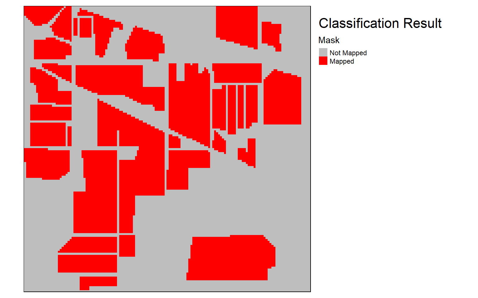
require(tmap)
tm_shape(raster_result)+
tm_raster(style= "cat", labels = c("Alfalfa","Corn","Grass","Hay","Oats","Soybeans","Trees","Wheat"),
palette = c("cyan4", "cornsilk", "darkgoldenrod3", "bisque4", "chocolate", "burlywood", "darkolivegreen", "darksalmon"),
title="Vegetation Types")+
tm_layout(title = "Classification Result", title.size = 1.5, title.snap.to.legend=TRUE)+
tm_layout(legend.outside=TRUE)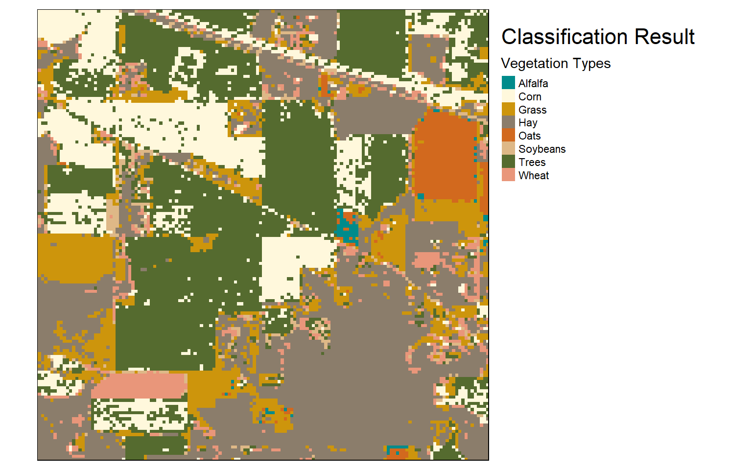
require(tmap)
tm_shape(result_masked)+
tm_raster(style= "cat", labels = c("Not Mapped", "Alfalfa","Corn","Grass","Hay","Oats","Soybeans","Trees","Wheat"),
palette = c("gray", "cyan4", "cornsilk", "darkgoldenrod3", "bisque4", "chocolate", "burlywood", "darkolivegreen", "darksalmon"),
title="Vegetation Types")+
tm_layout(title = "Classification Result", title.size = 1.5, title.snap.to.legend=TRUE)+
tm_layout(legend.outside=TRUE)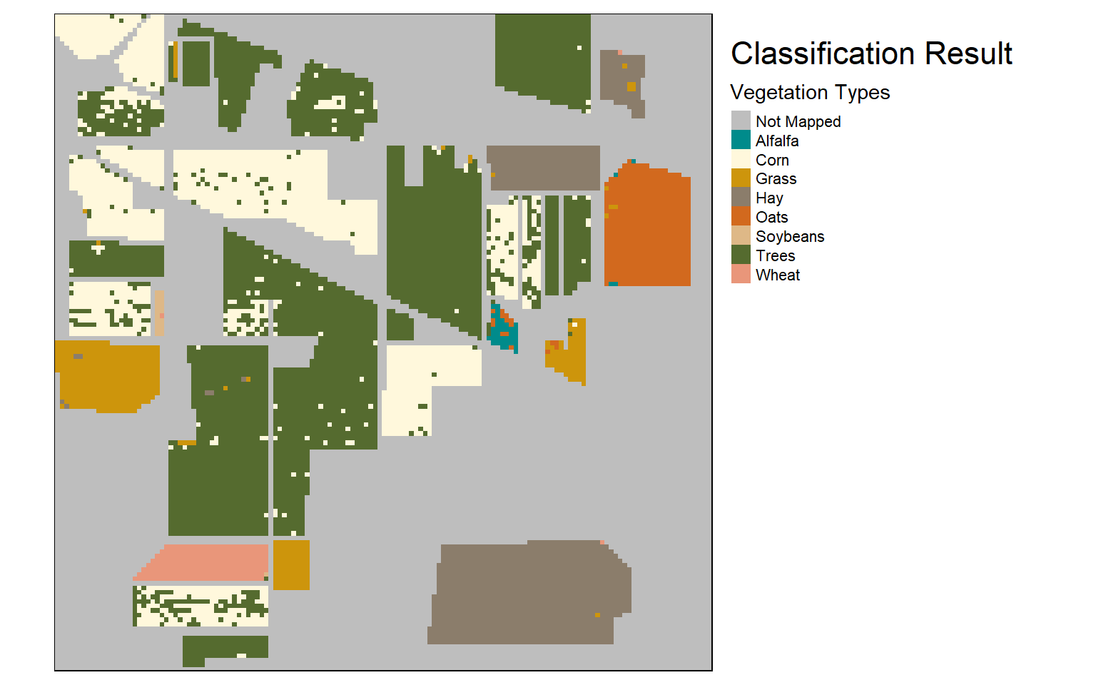
Example 3: Urban Land Cover Mapping using Machine learning and GEOBIA
In this example I will predict urban land cover types using predictor variables derived for image objects created using geographic object-based image analysis (GEOBIA). These data were obtained from the University of California, Irvine (UCI) Machine Learning Repository. The data were originally used in the following papers:
Johnson, B., and Xie, Z., 2013. Classifying a high resolution image of an urban area using super-object information. ISPRS Journal of Photogrammetry and Remote Sensing, 83, 40-49.
Johnson, B., 2013. High resolution urban land cover classification using a competitive multi-scale object-based approach. Remote Sensing Letters, 4 (2), 131-140.
The goal here is to differentiate urban land cover classes using multi-scale spectral, size, shape, and textural information calculated for each image object. Similar to the last example, the classes are imbalanced in the training and validation data sets.
In the first code block, I am reading in the data and counting the number of samples in each class in the training set.
train <- read.csv("caret/training.csv", header=TRUE, sep=",", stringsAsFactors=TRUE)
test <- read.csv("caret/testing.csv", header=TRUE, sep=",", stringsAsFactors=TRUE)

class_n <- train %>% dplyr::group_by(class) %>% dplyr::count()
print(class_n)
# A tibble: 9 x 2
# Groups:   class [9]
  class           n
  <fct>       <int>
1 "asphalt "     14
2 "building "    25
3 "car "         15
4 "concrete "    23
5 "grass "       29
6 "pool "        15
7 "shadow "      16
8 "soil "        14
9 "tree "        17
Similar to the above examples, I then tune and train the four different models. Here I am using 10-fold cross validation and optimizing relative to Kappa. Once the models are trained, I then use them to predict to the validation data. Lastly, I produce confusion matrices to assess and compare the results.
Take some time to review the results and assessment. Note that this is a different problem than those presented above; however, the syntax is very similar. This is one of the benefits of caret: it provides a standardized way to experiment with different algorithms and machine learning problems within R.
set.seed(42)
trainctrl <- trainControl(method = "cv", number = 10, verboseIter = FALSE)

knn.model <- train(class~., data=train, method = "knn",
tuneLength = 10,
preProcess = c("center", "scale"),
trControl = trainctrl,
metric="Kappa")

set.seed(42)
dt.model <- train(class~., data=train, method = "rpart",
tuneLength = 10,
preProcess = c("center", "scale"),
trControl = trainctrl,
metric="Kappa")

set.seed(42)
rf.model <- train(class~., data=train, method = "rf",
tuneLength = 10,
ntree = 100,
preProcess = c("center", "scale"),
trControl = trainctrl,
metric="Kappa")

svm.model <- train(class~., data=train, method = "svmRadial",
tuneLength = 10,
preProcess = c("center", "scale"),
trControl = trainctrl,
metric="Kappa")

knn.predict <-predict(knn.model, test)
dt.predict <-predict(dt.model, test)
rf.predict <- predict(rf.model, test)
svm.predict <-predict(svm.model, test)confusionMatrix(knn.predict, test$class)
Confusion Matrix and Statistics
Reference
Prediction asphalt building car concrete grass pool shadow soil tree
asphalt 34 0 0 0 0 0 9 0 0
building 0 68 1 4 1 1 0 2 0
car 0 0 14 1 0 0 0 0 0
concrete 1 19 0 71 5 0 0 3 0
grass 1 1 1 2 58 1 0 10 9
pool 0 1 1 0 0 12 2 0 0
shadow 6 2 0 0 0 0 31 0 2
soil 0 5 3 13 1 0 0 5 0
tree 3 1 1 2 18 0 3 0 78
Overall Statistics
Accuracy : 0.7318
95% CI : (0.6909, 0.7699)
No Information Rate : 0.1913
P-Value [Acc > NIR] : < 2.2e-16
Kappa : 0.6854
Mcnemar's Test P-Value : NA
Statistics by Class:
Class: asphalt Class: building Class: car
Sensitivity 0.75556 0.7010 0.66667
Specificity 0.98052 0.9780 0.99794
Pos Pred Value 0.79070 0.8831 0.93333
Neg Pred Value 0.97629 0.9326 0.98577
Prevalence 0.08876 0.1913 0.04142
Detection Rate 0.06706 0.1341 0.02761
Detection Prevalence 0.08481 0.1519 0.02959
Balanced Accuracy 0.86804 0.8395 0.83230
Class: concrete Class: grass Class: pool Class: shadow
Sensitivity 0.7634 0.6988 0.85714 0.68889
Specificity 0.9324 0.9410 0.99189 0.97835
Pos Pred Value 0.7172 0.6988 0.75000 0.75610
Neg Pred Value 0.9461 0.9410 0.99593 0.96996
Prevalence 0.1834 0.1637 0.02761 0.08876
Detection Rate 0.1400 0.1144 0.02367 0.06114
Detection Prevalence 0.1953 0.1637 0.03156 0.08087
Balanced Accuracy 0.8479 0.8199 0.92451 0.83362
Class: soil Class: tree
Sensitivity 0.250000 0.8764
Specificity 0.954825 0.9330
Pos Pred Value 0.185185 0.7358
Neg Pred Value 0.968750 0.9726
Prevalence 0.039448 0.1755
Detection Rate 0.009862 0.1538
Detection Prevalence 0.053254 0.2091
Balanced Accuracy 0.602413 0.9047confusionMatrix(dt.predict, test$class)
Confusion Matrix and Statistics
Reference
Prediction asphalt building car concrete grass pool shadow soil tree
asphalt 33 0 0 0 0 0 8 0 0
building 1 56 0 13 0 0 0 4 0
car 2 7 17 7 2 0 0 3 0
concrete 2 25 4 70 1 0 0 0 0
grass 0 0 0 0 73 1 0 0 35
pool 0 0 0 0 0 13 0 0 0
shadow 7 1 0 0 0 0 21 0 1
soil 0 8 0 3 3 0 0 13 0
tree 0 0 0 0 4 0 16 0 53
Overall Statistics
Accuracy : 0.6884
95% CI : (0.646, 0.7285)
No Information Rate : 0.1913
P-Value [Acc > NIR] : < 2.2e-16
Kappa : 0.6361
Mcnemar's Test P-Value : NA
Statistics by Class:
Class: asphalt Class: building Class: car
Sensitivity 0.73333 0.5773 0.80952
Specificity 0.98268 0.9561 0.95679
Pos Pred Value 0.80488 0.7568 0.44737
Neg Pred Value 0.97425 0.9053 0.99147
Prevalence 0.08876 0.1913 0.04142
Detection Rate 0.06509 0.1105 0.03353
Detection Prevalence 0.08087 0.1460 0.07495
Balanced Accuracy 0.85801 0.7667 0.88316
Class: concrete Class: grass Class: pool Class: shadow
Sensitivity 0.7527 0.8795 0.92857 0.46667
Specificity 0.9227 0.9151 1.00000 0.98052
Pos Pred Value 0.6863 0.6697 1.00000 0.70000
Neg Pred Value 0.9432 0.9749 0.99798 0.94969
Prevalence 0.1834 0.1637 0.02761 0.08876
Detection Rate 0.1381 0.1440 0.02564 0.04142
Detection Prevalence 0.2012 0.2150 0.02564 0.05917
Balanced Accuracy 0.8377 0.8973 0.96429 0.72359
Class: soil Class: tree
Sensitivity 0.65000 0.5955
Specificity 0.97125 0.9522
Pos Pred Value 0.48148 0.7260
Neg Pred Value 0.98542 0.9171
Prevalence 0.03945 0.1755
Detection Rate 0.02564 0.1045
Detection Prevalence 0.05325 0.1440
Balanced Accuracy 0.81063 0.7738confusionMatrix(rf.predict, test$class)
Confusion Matrix and Statistics
Reference
Prediction asphalt building car concrete grass pool shadow soil tree
asphalt 38 0 0 0 0 0 4 0 0
building 0 68 0 3 1 0 0 3 0
car 2 3 20 5 1 0 1 3 0
concrete 1 21 1 84 0 0 0 1 0
grass 0 0 0 0 70 1 0 0 23
pool 0 0 0 0 0 13 0 0 0
shadow 3 2 0 0 0 0 39 0 3
soil 1 3 0 1 4 0 0 13 0
tree 0 0 0 0 7 0 1 0 63
Overall Statistics
Accuracy : 0.8047
95% CI : (0.7675, 0.8384)
No Information Rate : 0.1913
P-Value [Acc > NIR] : < 2.2e-16
Kappa : 0.7721
Mcnemar's Test P-Value : NA
Statistics by Class:
Class: asphalt Class: building Class: car
Sensitivity 0.84444 0.7010 0.95238
Specificity 0.99134 0.9829 0.96914
Pos Pred Value 0.90476 0.9067 0.57143
Neg Pred Value 0.98495 0.9329 0.99788
Prevalence 0.08876 0.1913 0.04142
Detection Rate 0.07495 0.1341 0.03945
Detection Prevalence 0.08284 0.1479 0.06903
Balanced Accuracy 0.91789 0.8420 0.96076
Class: concrete Class: grass Class: pool Class: shadow
Sensitivity 0.9032 0.8434 0.92857 0.86667
Specificity 0.9420 0.9434 1.00000 0.98268
Pos Pred Value 0.7778 0.7447 1.00000 0.82979
Neg Pred Value 0.9774 0.9685 0.99798 0.98696
Prevalence 0.1834 0.1637 0.02761 0.08876
Detection Rate 0.1657 0.1381 0.02564 0.07692
Detection Prevalence 0.2130 0.1854 0.02564 0.09270
Balanced Accuracy 0.9226 0.8934 0.96429 0.92468
Class: soil Class: tree
Sensitivity 0.65000 0.7079
Specificity 0.98152 0.9809
Pos Pred Value 0.59091 0.8873
Neg Pred Value 0.98557 0.9404
Prevalence 0.03945 0.1755
Detection Rate 0.02564 0.1243
Detection Prevalence 0.04339 0.1400
Balanced Accuracy 0.81576 0.8444confusionMatrix(svm.predict, test$class)
Confusion Matrix and Statistics
Reference
Prediction asphalt building car concrete grass pool shadow soil tree
asphalt 32 1 0 0 0 0 2 0 0
building 0 72 0 7 1 2 0 2 0
car 0 3 20 5 0 0 0 1 1
concrete 1 16 0 73 1 0 0 3 0
grass 0 1 0 0 63 1 0 6 16
pool 0 1 0 0 0 11 2 0 0
shadow 12 1 0 0 0 0 41 0 3
soil 0 2 1 7 5 0 0 8 0
tree 0 0 0 1 13 0 0 0 69
Overall Statistics
Accuracy : 0.7673
95% CI : (0.728, 0.8034)
No Information Rate : 0.1913
P-Value [Acc > NIR] : < 2.2e-16
Kappa : 0.7282
Mcnemar's Test P-Value : NA
Statistics by Class:
Class: asphalt Class: building Class: car
Sensitivity 0.71111 0.7423 0.95238
Specificity 0.99351 0.9707 0.97942
Pos Pred Value 0.91429 0.8571 0.66667
Neg Pred Value 0.97246 0.9409 0.99790
Prevalence 0.08876 0.1913 0.04142
Detection Rate 0.06312 0.1420 0.03945
Detection Prevalence 0.06903 0.1657 0.05917
Balanced Accuracy 0.85231 0.8565 0.96590
Class: concrete Class: grass Class: pool Class: shadow
Sensitivity 0.7849 0.7590 0.78571 0.91111
Specificity 0.9493 0.9434 0.99391 0.96537
Pos Pred Value 0.7766 0.7241 0.78571 0.71930
Neg Pred Value 0.9516 0.9524 0.99391 0.99111
Prevalence 0.1834 0.1637 0.02761 0.08876
Detection Rate 0.1440 0.1243 0.02170 0.08087
Detection Prevalence 0.1854 0.1716 0.02761 0.11243
Balanced Accuracy 0.8671 0.8512 0.88981 0.93824
Class: soil Class: tree
Sensitivity 0.40000 0.7753
Specificity 0.96920 0.9665
Pos Pred Value 0.34783 0.8313
Neg Pred Value 0.97521 0.9528
Prevalence 0.03945 0.1755
Detection Rate 0.01578 0.1361
Detection Prevalence 0.04536 0.1637
Balanced Accuracy 0.68460 0.8709As noted in the machine learning background lectures, algorithms can be negatively impacted by imbalance in the training data. Fortunately, caret has built-in techniques for dealing with this issue including the following:
Down-Sampling (“down”): randomly down-sample more prevalent classes so that they have the same or a similar number of samples as the least frequent class
Up-sampling (“up”): randomly up-sample or duplicate samples from the least frequent classes
SMOTE (“smote”): down-sample the majority class and synthesizes new minority instances by interpolating between existing ones (synthetic minority sampling techniques)
In this example, I am using the up-sampling method. Notice that the code is the same as the example above, except that I have added sampling=“up” to the training controls. So, this is an easy experiment to perform. Compare the obtained results to those obtained without up-sampling. Did this provide any improvement? Are minority classes now being mapped more accurately? Note the impact of data balancing will vary based on the specific classification problem. So, you may or may not observe improvement.
set.seed(420)
trainctrl <- trainControl(method = "cv", number = 10, sampling="up", verboseIter = FALSE)

knn.model <- train(class~., data=train, method = "knn",
tuneLength = 10,
preProcess = c("center", "scale"),
trControl = trainctrl,
metric="Kappa")

set.seed(42)
dt.model <- train(class~., data=train, method = "rpart",
tuneLength = 10,
preProcess = c("center", "scale"),
trControl = trainctrl,
metric="Kappa")

set.seed(42)
rf.model <- train(class~., data=train, method = "rf",
tuneLength = 10,
ntree = 100,
preProcess = c("center", "scale"),
trControl = trainctrl,
metric="Kappa")

svm.model <- train(class~., data=train, method = "svmRadial",
tuneLength = 10,
preProcess = c("center", "scale"),
trControl = trainctrl,
metric="Kappa")

knn.predict <-predict(knn.model, test)
dt.predict <-predict(dt.model, test)
rf.predict <- predict(rf.model, test)
svm.predict <-predict(svm.model, test)confusionMatrix(knn.predict, test$class)
Confusion Matrix and Statistics
Reference
Prediction asphalt building car concrete grass pool shadow soil tree
asphalt 35 0 0 0 0 0 10 0 0
building 0 67 1 3 1 1 0 3 0
car 0 0 14 1 0 0 0 0 0
concrete 0 12 0 47 3 0 0 3 0
grass 0 1 0 1 46 0 0 4 1
pool 0 1 2 0 0 12 3 0 0
shadow 8 2 0 0 0 0 30 0 4
soil 1 13 4 40 6 0 0 10 0
tree 1 1 0 1 27 1 2 0 84
Overall Statistics
Accuracy : 0.6805
95% CI : (0.6379, 0.7209)
No Information Rate : 0.1913
P-Value [Acc > NIR] : < 2.2e-16
Kappa : 0.6313
Mcnemar's Test P-Value : NA
Statistics by Class:
Class: asphalt Class: building Class: car
Sensitivity 0.77778 0.6907 0.66667
Specificity 0.97835 0.9780 0.99794
Pos Pred Value 0.77778 0.8816 0.93333
Neg Pred Value 0.97835 0.9304 0.98577
Prevalence 0.08876 0.1913 0.04142
Detection Rate 0.06903 0.1321 0.02761
Detection Prevalence 0.08876 0.1499 0.02959
Balanced Accuracy 0.87807 0.8344 0.83230
Class: concrete Class: grass Class: pool Class: shadow
Sensitivity 0.5054 0.55422 0.85714 0.66667
Specificity 0.9565 0.98349 0.98783 0.96970
Pos Pred Value 0.7231 0.86792 0.66667 0.68182
Neg Pred Value 0.8959 0.91850 0.99591 0.96760
Prevalence 0.1834 0.16371 0.02761 0.08876
Detection Rate 0.0927 0.09073 0.02367 0.05917
Detection Prevalence 0.1282 0.10454 0.03550 0.08679
Balanced Accuracy 0.7309 0.76885 0.92249 0.81818
Class: soil Class: tree
Sensitivity 0.50000 0.9438
Specificity 0.86858 0.9211
Pos Pred Value 0.13514 0.7179
Neg Pred Value 0.97691 0.9872
Prevalence 0.03945 0.1755
Detection Rate 0.01972 0.1657
Detection Prevalence 0.14596 0.2308
Balanced Accuracy 0.68429 0.9324confusionMatrix(dt.predict, test$class)
Confusion Matrix and Statistics
Reference
Prediction asphalt building car concrete grass pool shadow soil tree
asphalt 29 0 0 0 0 0 7 0 0
building 1 56 0 13 0 0 1 4 0
car 4 7 17 7 2 0 1 2 1
concrete 4 25 4 70 1 0 0 0 0
grass 0 0 0 0 51 0 0 0 7
pool 0 0 0 0 0 13 0 0 0
shadow 7 1 0 0 2 0 34 0 8
soil 0 8 0 3 5 0 0 13 0
tree 0 0 0 0 22 1 2 1 73
Overall Statistics
Accuracy : 0.7022
95% CI : (0.6603, 0.7417)
No Information Rate : 0.1913
P-Value [Acc > NIR] : < 2.2e-16
Kappa : 0.6534
Mcnemar's Test P-Value : NA
Statistics by Class:
Class: asphalt Class: building Class: car
Sensitivity 0.64444 0.5773 0.80952
Specificity 0.98485 0.9537 0.95062
Pos Pred Value 0.80556 0.7467 0.41463
Neg Pred Value 0.96603 0.9051 0.99142
Prevalence 0.08876 0.1913 0.04142
Detection Rate 0.05720 0.1105 0.03353
Detection Prevalence 0.07101 0.1479 0.08087
Balanced Accuracy 0.81465 0.7655 0.88007
Class: concrete Class: grass Class: pool Class: shadow
Sensitivity 0.7527 0.6145 0.92857 0.75556
Specificity 0.9179 0.9835 1.00000 0.96104
Pos Pred Value 0.6731 0.8793 1.00000 0.65385
Neg Pred Value 0.9429 0.9287 0.99798 0.97582
Prevalence 0.1834 0.1637 0.02761 0.08876
Detection Rate 0.1381 0.1006 0.02564 0.06706
Detection Prevalence 0.2051 0.1144 0.02564 0.10256
Balanced Accuracy 0.8353 0.7990 0.96429 0.85830
Class: soil Class: tree
Sensitivity 0.65000 0.8202
Specificity 0.96715 0.9378
Pos Pred Value 0.44828 0.7374
Neg Pred Value 0.98536 0.9608
Prevalence 0.03945 0.1755
Detection Rate 0.02564 0.1440
Detection Prevalence 0.05720 0.1953
Balanced Accuracy 0.80857 0.8790confusionMatrix(rf.predict, test$class)
Confusion Matrix and Statistics
Reference
Prediction asphalt building car concrete grass pool shadow soil tree
asphalt 33 1 0 0 0 0 2 0 0
building 0 72 0 4 1 1 0 3 0
car 1 5 20 3 1 0 0 1 1
concrete 0 15 1 82 0 0 0 2 0
grass 2 1 0 2 68 0 0 6 16
pool 0 0 0 0 0 12 2 0 0
shadow 7 1 0 0 0 0 40 0 4
soil 0 2 0 1 1 0 0 8 0
tree 2 0 0 1 12 1 1 0 68
Overall Statistics
Accuracy : 0.7949
95% CI : (0.7571, 0.8292)
No Information Rate : 0.1913
P-Value [Acc > NIR] : < 2.2e-16
Kappa : 0.7596
Mcnemar's Test P-Value : NA
Statistics by Class:
Class: asphalt Class: building Class: car
Sensitivity 0.73333 0.7423 0.95238
Specificity 0.99351 0.9780 0.97531
Pos Pred Value 0.91667 0.8889 0.62500
Neg Pred Value 0.97452 0.9413 0.99789
Prevalence 0.08876 0.1913 0.04142
Detection Rate 0.06509 0.1420 0.03945
Detection Prevalence 0.07101 0.1598 0.06312
Balanced Accuracy 0.86342 0.8602 0.96384
Class: concrete Class: grass Class: pool Class: shadow
Sensitivity 0.8817 0.8193 0.85714 0.88889
Specificity 0.9565 0.9363 0.99594 0.97403
Pos Pred Value 0.8200 0.7158 0.85714 0.76923
Neg Pred Value 0.9730 0.9636 0.99594 0.98901
Prevalence 0.1834 0.1637 0.02761 0.08876
Detection Rate 0.1617 0.1341 0.02367 0.07890
Detection Prevalence 0.1972 0.1874 0.02761 0.10256
Balanced Accuracy 0.9191 0.8778 0.92654 0.93146
Class: soil Class: tree
Sensitivity 0.40000 0.7640
Specificity 0.99179 0.9593
Pos Pred Value 0.66667 0.8000
Neg Pred Value 0.97576 0.9502
Prevalence 0.03945 0.1755
Detection Rate 0.01578 0.1341
Detection Prevalence 0.02367 0.1677
Balanced Accuracy 0.69589 0.8617confusionMatrix(svm.predict, test$class)
Confusion Matrix and Statistics
Reference
Prediction asphalt building car concrete grass pool shadow soil tree
asphalt 31 0 0 0 0 0 4 0 0
building 0 69 0 6 1 1 0 2 0
car 1 1 20 4 1 0 0 1 3
concrete 1 15 0 62 2 0 0 3 1
grass 0 1 0 0 56 0 0 6 9
pool 0 1 0 0 0 12 1 0 0
shadow 12 2 0 0 0 0 40 0 3
soil 0 8 1 20 8 0 0 8 0
tree 0 0 0 1 15 1 0 0 73
Overall Statistics
Accuracy : 0.7318
95% CI : (0.6909, 0.7699)
No Information Rate : 0.1913
P-Value [Acc > NIR] : < 2.2e-16
Kappa : 0.689
Mcnemar's Test P-Value : NA
Statistics by Class:
Class: asphalt Class: building Class: car
Sensitivity 0.68889 0.7113 0.95238
Specificity 0.99134 0.9756 0.97737
Pos Pred Value 0.88571 0.8734 0.64516
Neg Pred Value 0.97034 0.9346 0.99790
Prevalence 0.08876 0.1913 0.04142
Detection Rate 0.06114 0.1361 0.03945
Detection Prevalence 0.06903 0.1558 0.06114
Balanced Accuracy 0.84012 0.8435 0.96487
Class: concrete Class: grass Class: pool Class: shadow
Sensitivity 0.6667 0.6747 0.85714 0.88889
Specificity 0.9469 0.9623 0.99594 0.96320
Pos Pred Value 0.7381 0.7778 0.85714 0.70175
Neg Pred Value 0.9267 0.9379 0.99594 0.98889
Prevalence 0.1834 0.1637 0.02761 0.08876
Detection Rate 0.1223 0.1105 0.02367 0.07890
Detection Prevalence 0.1657 0.1420 0.02761 0.11243
Balanced Accuracy 0.8068 0.8185 0.92654 0.92605
Class: soil Class: tree
Sensitivity 0.40000 0.8202
Specificity 0.92402 0.9593
Pos Pred Value 0.17778 0.8111
Neg Pred Value 0.97403 0.9616
Prevalence 0.03945 0.1755
Detection Rate 0.01578 0.1440
Detection Prevalence 0.08876 0.1775
Balanced Accuracy 0.66201 0.8898In this last example I am including feature selection using rfeControls and a random forest-based feature selection method. I am testing multiple subset sizes (from 1 to 147 variables by steps of 5 variables). Once the feature selection is complete, I then subset out the selected variables then create predictions using only this subset.
Again, whether or not feature selection improves model performance depends on the specific problem and varies on a case-by-case basis. Compare the obtained results. How did these models perform in comparison to the original models and balanced models? What variables were found to be important?
set.seed(42)
trainctrl <- trainControl(method = "cv", number = 10, verboseIter = FALSE)

set.seed(42)
fsctrl <- rfeControl(functions=rfFuncs, method="cv", number=10)
to_test <- seq(1, 147, by=5)

set.seed(42)
fs_result <- rfe(train[,2:ncol(train)], train[,1], sizes=c(to_test), metric = "Kappa", rfeControl=fsctrl)
selected <- predictors(fs_result)

#Prepare training and test data
test2 <- test[,selected]
test3 <- cbind(test$class, test2)
colnames(test3)[1] <- "class"
testx <- as.data.frame(test3)
train2 <- train[,selected]
train3 <- cbind(train$class, train2)
colnames(train3)[1] <- "class"
trainx <- as.data.frame(train3)


knn.model <- train(class~., data=trainx, method = "knn",
tuneLength = 10,
preProcess = c("center", "scale"),
trControl = trainctrl,
metric="Kappa")

set.seed(42)
dt.model <- train(class~., data=trainx, method = "rpart",
tuneLength = 10,
preProcess = c("center", "scale"),
trControl = trainctrl,
metric="Kappa")

set.seed(42)
rf.model <- train(class~., data=trainx, method = "rf",
tuneLength = 10,
ntree = 100,
preProcess = c("center", "scale"),
trControl = trainctrl,
metric="Kappa")

svm.model <- train(class~., data=trainx, method = "svmRadial",
tuneLength = 10,
preProcess = c("center", "scale"),
trControl = trainctrl,
metric="Kappa")

knn.predict <-predict(knn.model, testx)
dt.predict <-predict(dt.model, testx)
rf.predict <- predict(rf.model, testx)
svm.predict <-predict(svm.model, test)confusionMatrix(knn.predict, testx$class)
Confusion Matrix and Statistics
Reference
Prediction asphalt building car concrete grass pool shadow soil tree
asphalt 34 1 0 0 0 0 6 0 0
building 0 66 1 5 0 2 0 2 0
car 0 0 15 2 1 0 0 0 0
concrete 0 22 0 70 3 0 0 1 0
grass 1 0 0 1 62 1 0 6 10
pool 0 1 1 0 0 11 2 0 0
shadow 9 1 0 0 0 0 35 0 6
soil 0 5 3 14 2 0 0 11 0
tree 1 1 1 1 15 0 2 0 73
Overall Statistics
Accuracy : 0.7436
95% CI : (0.7032, 0.7811)
No Information Rate : 0.1913
P-Value [Acc > NIR] : < 2.2e-16
Kappa : 0.7007
Mcnemar's Test P-Value : NA
Statistics by Class:
Class: asphalt Class: building Class: car
Sensitivity 0.75556 0.6804 0.71429
Specificity 0.98485 0.9756 0.99383
Pos Pred Value 0.82927 0.8684 0.83333
Neg Pred Value 0.97639 0.9281 0.98773
Prevalence 0.08876 0.1913 0.04142
Detection Rate 0.06706 0.1302 0.02959
Detection Prevalence 0.08087 0.1499 0.03550
Balanced Accuracy 0.87020 0.8280 0.85406
Class: concrete Class: grass Class: pool Class: shadow
Sensitivity 0.7527 0.7470 0.78571 0.77778
Specificity 0.9372 0.9552 0.99189 0.96537
Pos Pred Value 0.7292 0.7654 0.73333 0.68627
Neg Pred Value 0.9440 0.9507 0.99390 0.97807
Prevalence 0.1834 0.1637 0.02761 0.08876
Detection Rate 0.1381 0.1223 0.02170 0.06903
Detection Prevalence 0.1893 0.1598 0.02959 0.10059
Balanced Accuracy 0.8449 0.8511 0.88880 0.87157
Class: soil Class: tree
Sensitivity 0.55000 0.8202
Specificity 0.95072 0.9498
Pos Pred Value 0.31429 0.7766
Neg Pred Value 0.98093 0.9613
Prevalence 0.03945 0.1755
Detection Rate 0.02170 0.1440
Detection Prevalence 0.06903 0.1854
Balanced Accuracy 0.75036 0.8850confusionMatrix(dt.predict, testx$class)
Confusion Matrix and Statistics
Reference
Prediction asphalt building car concrete grass pool shadow soil tree
asphalt 33 0 0 0 0 0 8 0 0
building 1 56 0 13 0 0 0 4 0
car 2 7 17 7 2 0 0 3 0
concrete 2 25 4 70 1 0 0 0 0
grass 0 0 0 0 73 1 0 0 35
pool 0 0 0 0 0 13 0 0 0
shadow 7 1 0 0 0 0 21 0 1
soil 0 8 0 3 3 0 0 13 0
tree 0 0 0 0 4 0 16 0 53
Overall Statistics
Accuracy : 0.6884
95% CI : (0.646, 0.7285)
No Information Rate : 0.1913
P-Value [Acc > NIR] : < 2.2e-16
Kappa : 0.6361
Mcnemar's Test P-Value : NA
Statistics by Class:
Class: asphalt Class: building Class: car
Sensitivity 0.73333 0.5773 0.80952
Specificity 0.98268 0.9561 0.95679
Pos Pred Value 0.80488 0.7568 0.44737
Neg Pred Value 0.97425 0.9053 0.99147
Prevalence 0.08876 0.1913 0.04142
Detection Rate 0.06509 0.1105 0.03353
Detection Prevalence 0.08087 0.1460 0.07495
Balanced Accuracy 0.85801 0.7667 0.88316
Class: concrete Class: grass Class: pool Class: shadow
Sensitivity 0.7527 0.8795 0.92857 0.46667
Specificity 0.9227 0.9151 1.00000 0.98052
Pos Pred Value 0.6863 0.6697 1.00000 0.70000
Neg Pred Value 0.9432 0.9749 0.99798 0.94969
Prevalence 0.1834 0.1637 0.02761 0.08876
Detection Rate 0.1381 0.1440 0.02564 0.04142
Detection Prevalence 0.2012 0.2150 0.02564 0.05917
Balanced Accuracy 0.8377 0.8973 0.96429 0.72359
Class: soil Class: tree
Sensitivity 0.65000 0.5955
Specificity 0.97125 0.9522
Pos Pred Value 0.48148 0.7260
Neg Pred Value 0.98542 0.9171
Prevalence 0.03945 0.1755
Detection Rate 0.02564 0.1045
Detection Prevalence 0.05325 0.1440
Balanced Accuracy 0.81063 0.7738confusionMatrix(rf.predict, testx$class)
Confusion Matrix and Statistics
Reference
Prediction asphalt building car concrete grass pool shadow soil tree
asphalt 36 1 0 0 0 0 1 0 0
building 1 67 0 7 0 2 0 1 0
car 1 3 20 3 1 0 0 1 0
concrete 0 23 1 80 1 0 0 1 0
grass 1 0 0 0 75 1 0 6 17
pool 0 0 0 0 0 11 1 0 0
shadow 5 1 0 0 0 0 42 0 7
soil 0 2 0 2 1 0 0 11 0
tree 1 0 0 1 5 0 1 0 65
Overall Statistics
Accuracy : 0.8028
95% CI : (0.7654, 0.8365)
No Information Rate : 0.1913
P-Value [Acc > NIR] : < 2.2e-16
Kappa : 0.7691
Mcnemar's Test P-Value : NA
Statistics by Class:
Class: asphalt Class: building Class: car
Sensitivity 0.80000 0.6907 0.95238
Specificity 0.99567 0.9732 0.98148
Pos Pred Value 0.94737 0.8590 0.68966
Neg Pred Value 0.98081 0.9301 0.99791
Prevalence 0.08876 0.1913 0.04142
Detection Rate 0.07101 0.1321 0.03945
Detection Prevalence 0.07495 0.1538 0.05720
Balanced Accuracy 0.89784 0.8319 0.96693
Class: concrete Class: grass Class: pool Class: shadow
Sensitivity 0.8602 0.9036 0.78571 0.93333
Specificity 0.9372 0.9410 0.99797 0.97186
Pos Pred Value 0.7547 0.7500 0.91667 0.76364
Neg Pred Value 0.9676 0.9803 0.99394 0.99336
Prevalence 0.1834 0.1637 0.02761 0.08876
Detection Rate 0.1578 0.1479 0.02170 0.08284
Detection Prevalence 0.2091 0.1972 0.02367 0.10848
Balanced Accuracy 0.8987 0.9223 0.89184 0.95260
Class: soil Class: tree
Sensitivity 0.55000 0.7303
Specificity 0.98973 0.9809
Pos Pred Value 0.68750 0.8904
Neg Pred Value 0.98167 0.9447
Prevalence 0.03945 0.1755
Detection Rate 0.02170 0.1282
Detection Prevalence 0.03156 0.1440
Balanced Accuracy 0.76987 0.8556confusionMatrix(svm.predict, testx$class)
Confusion Matrix and Statistics
Reference
Prediction asphalt building car concrete grass pool shadow soil tree
asphalt 32 0 0 0 0 0 1 0 0
building 0 67 0 5 0 1 0 2 0
car 1 3 20 5 2 0 1 1 1
concrete 0 24 0 79 2 0 0 3 0
grass 1 0 0 0 65 1 0 6 11
pool 0 0 0 0 0 12 1 0 0
shadow 11 2 0 0 0 0 42 0 6
soil 0 1 1 3 2 0 0 8 0
tree 0 0 0 1 12 0 0 0 71
Overall Statistics
Accuracy : 0.7811
95% CI : (0.7425, 0.8163)
No Information Rate : 0.1913
P-Value [Acc > NIR] : < 2.2e-16
Kappa : 0.744
Mcnemar's Test P-Value : NA
Statistics by Class:
Class: asphalt Class: building Class: car
Sensitivity 0.71111 0.6907 0.95238
Specificity 0.99784 0.9805 0.97119
Pos Pred Value 0.96970 0.8933 0.58824
Neg Pred Value 0.97257 0.9306 0.99789
Prevalence 0.08876 0.1913 0.04142
Detection Rate 0.06312 0.1321 0.03945
Detection Prevalence 0.06509 0.1479 0.06706
Balanced Accuracy 0.85447 0.8356 0.96179
Class: concrete Class: grass Class: pool Class: shadow
Sensitivity 0.8495 0.7831 0.85714 0.93333
Specificity 0.9300 0.9552 0.99797 0.95887
Pos Pred Value 0.7315 0.7738 0.92308 0.68852
Neg Pred Value 0.9649 0.9574 0.99595 0.99327
Prevalence 0.1834 0.1637 0.02761 0.08876
Detection Rate 0.1558 0.1282 0.02367 0.08284
Detection Prevalence 0.2130 0.1657 0.02564 0.12032
Balanced Accuracy 0.8897 0.8692 0.92756 0.94610
Class: soil Class: tree
Sensitivity 0.40000 0.7978
Specificity 0.98563 0.9689
Pos Pred Value 0.53333 0.8452
Neg Pred Value 0.97561 0.9574
Prevalence 0.03945 0.1755
Detection Rate 0.01578 0.1400
Detection Prevalence 0.02959 0.1657
Balanced Accuracy 0.69281 0.8833Example 4: A Regression Example
It is also possible to use caret to produce continuous predictions, similar to linear regression and geographically weighted regression. In this last example, I will repeat a portion of the analysis from the regression module and compare the results to those obtained with machine learning. As you might remember, the goal is to predict the percentage of people over 25 that have at least a bachelors degree by county using multiple other variables. This data violated several assumptions of linear regression, so machine learning might be more appropriate.
First, I read in the Census data as a table. Then I split the data into training and testing sets using a 50/50 split. I make a model using multiple regression then predict to the withheld data and obtain an RMSE estimate.
Next, I create models and predictions using the four machine learning algorithms. Note that I have changed the tuning metric to RMSE, as Kappa is not appropriate for a continuous prediction. I then predict to the withheld data and obtain RMSE values.
In the last two code blocks, I generate a graph to compare the RMSE values. Based on RMSE, all the machine learning methods outperformed multiple regression. Random forests and support vector machines provide the best performance.
census <- read.csv("caret/census_data.csv", sep=",", header=TRUE, stringsAsFactors=TRUE)set.seed(42)
train_reg <- census %>% sample_frac(0.5)
test_reg <- setdiff(census, train_reg)mr_model <- lm(per_25_bach ~ per_no_hus + per_with_child_u18 + avg_fam_size + per_fem_div_15 + per_native_born + per_eng_only + per_broadband, data = train_reg)mr_predict <- predict(mr_model, test_reg)
mr_rmse <- rmse(test_reg$per_25_bach, mr_predict)set.seed(42)
trainctrl <- trainControl(method = "cv", number = 10, verboseIter = FALSE)
knn.model <- train(per_25_bach ~ per_no_hus + per_with_child_u18 + avg_fam_size + per_fem_div_15 + per_native_born + per_eng_only + per_broadband, data = train_reg, method = "knn",
tuneLength = 10,
preProcess = c("center", "scale"),
trControl = trainctrl,
metric="RMSE")
set.seed(42)
dt.model <- train(per_25_bach ~ per_no_hus + per_with_child_u18 + avg_fam_size + per_fem_div_15 + per_native_born + per_eng_only + per_broadband, data = train_reg, method = "rpart",
tuneLength = 10,
preProcess = c("center", "scale"),
trControl = trainctrl,
metric="RMSE")
set.seed(42)
rf.model <- train(per_25_bach ~ per_no_hus + per_with_child_u18 + avg_fam_size + per_fem_div_15 + per_native_born + per_eng_only + per_broadband, data = train_reg, method = "rf",
tuneLength = 10,
ntree = 100,
preProcess = c("center", "scale"),
trControl = trainctrl,
metric="RMSE")
note: only 6 unique complexity parameters in default grid. Truncating the grid to 6 .
svm.model <- train(per_25_bach ~ per_no_hus + per_with_child_u18 + avg_fam_size + per_fem_div_15 + per_native_born + per_eng_only + per_broadband, data = train_reg, method = "svmRadial",
tuneLength = 10,
preProcess = c("center", "scale"),
trControl = trainctrl,
metric="RMSE")
knn.predict <-predict(knn.model, test_reg)
dt.predict <-predict(dt.model, test_reg)
rf.predict <- predict(rf.model, test_reg)
svm.predict <-predict(svm.model, test_reg)
knn_rmse <- rmse(test_reg$per_25_bach, knn.predict)
dt_rmse <- rmse(test_reg$per_25_bach, dt.predict)
rf_rmse <- rmse(test_reg$per_25_bach, rf.predict)
svm_rmse <- rmse(test_reg$per_25_bach, svm.predict)rmse_results <- c(mr_rmse, knn_rmse, dt_rmse, rf_rmse, svm_rmse)
rmse_labels <- c("Multiple Regression", "k-NN", "Decision Trees", "Random Forest", "Support Vector Machines")
rmse_data <- data.frame(model=rmse_labels, rmse=rmse_results)ggplot(rmse_data, aes(x=reorder(model, rmse), y=rmse))+
geom_bar(stat="identity")+
ggtitle("Model Comparison")+
labs(x="RMSE", y="Model")+
coord_flip()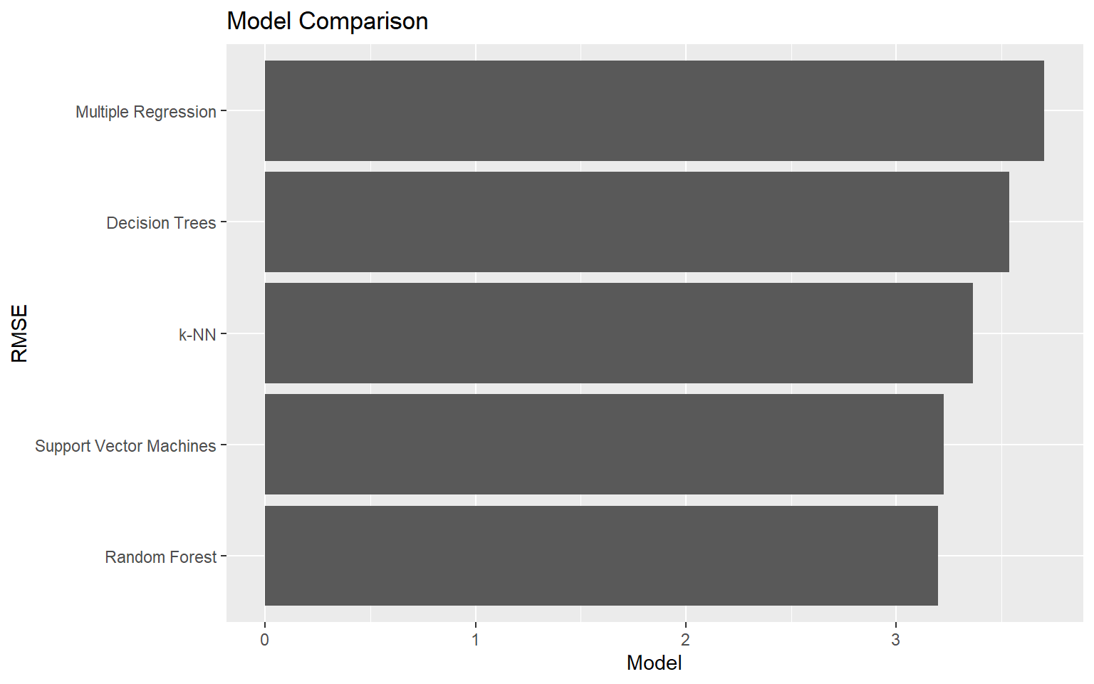
Concluding Remarks
That’s it! Using these examples, you should be able to apply machine learning to make predictions on spatial data. I would recommend trying out these methods on your own data and experimenting with different algorithms.