| Characteristic | Generalized Additive Model (GAM) | Explainable Boosting Machine (EBM) |
|---|---|---|
| Shape functions | Smooth splines (penalized regression splines) | Piecewise constant (step) functions learned with shallow trees |
| How shapes are learned | Penalized likelihood; smoothness selected with REML | Cyclic gradient boosting with a small learning rate and bagging |
| Smoothness | Controlled by a penalty; effective degrees of freedom (edf) summarize complexity | Controlled by the number of bins and boosting rounds; can capture abrupt changes |
| Uncertainty | Confidence intervals and approximate p-values for each smooth term | No standard errors in the R package |
| Interactions | Supported with tensor product smooths (e.g. te()) | Pairwise interactions supported in Python; not in the R package |
| Tasks in R | Regression, classification, counts, and many other distributions | Binary classification only |
| R package | mgcv | interpret |
11 Interpretable Models (GAMs and EBMs)
11.1 Topics Covered
- Interpretable (“glass-box”) models versus post hoc explanations
- The additive model structure
- Training and interpreting generalized additive models (GAMs) with mgcv and gratia
- Checking GAMs: basis dimension and concurvity
- Training and interpreting explainable boosting machines (EBMs) with interpret
- Explaining individual predictions with additive models
- Comparing shape functions learned by different models
11.2 Introduction
In Chapter 10, we used random forest to map the likelihood of palustrine forested/palustrine scrub/shrub (PFO/PSS) wetland occurrence. Random forest performed well, but it is a “black-box” model: its predictions are generated by hundreds of deep decision trees, so we cannot directly see how the predictor variables are used. Instead, we relied on post hoc methods, such as permutation-based variable importance, partial dependence plots, and SHAP values, to approximate how the model behaves. These explanations are useful, but they are approximations of the model, not the model itself, and they can be misleading when predictor variables are correlated.
An alternative is to use a model that is interpretable by design, sometimes called a glass-box model. In this chapter, we explore two such models: generalized additive models (GAMs) and explainable boosting machines (EBMs). Both have the same additive structure:
\[g(E[y]) = \beta_0 + f_1(x_1) + f_2(x_2) + \dots + f_p(x_p)\]
where \(g()\) is a link function, \(\beta_0\) is an intercept, and each \(f_j()\) is a shape function that describes how predictor variable \(x_j\) contributes to the prediction. For binary classification, as in our wetland problem, the link function is the logit, so the model predicts the log-odds of the class of interest:
\[\log\left(\frac{p}{1-p}\right) = \beta_0 + f_1(x_1) + f_2(x_2) + \dots + f_p(x_p)\]
This should look familiar. Logistic regression, which was compared to random forest in Chapter 10, has the same structure, except that each shape function is restricted to a straight line: \(f_j(x_j) = \beta_j x_j\). GAMs and EBMs relax this restriction and allow each shape function to be non-linear, which can greatly improve predictive performance. Importantly, since the model is still a sum of separate functions, each of which depends on a single predictor variable, the shape functions are the model. Plotting them shows exactly how each predictor variable is used, and the prediction for any location can be decomposed exactly into the contribution of each predictor variable.
GAMs and EBMs differ in how the shape functions are learned, as summarized in Table 11.1. A GAM represents each shape function as a smooth function constructed from a set of basis functions, or splines. To avoid overfitting, a penalty is applied to the “wiggliness” of each learned function, and the strength of the penalty is estimated from the data. An EBM learns each shape function using gradient boosting with very shallow decision trees. Instead of building trees that use many predictor variables, an EBM cycles through the predictor variables one at a time, fitting a tiny tree to the current residuals using only that predictor variable, with a very small learning rate. This is repeated thousands of times and averaged over multiple bagged models. The result is a step-like shape function for each predictor variable.
We fit GAMs using the mgcv package, which is the most widely used and fully featured implementation of GAMs in R, and visualize them using gratia, which produces ggplot2-based plots of mgcv models. EBMs are fit using the interpret package, which is the R interface to the InterpretML library developed by Microsoft Research. Note that the R version of interpret currently only supports binary classification; it cannot be used for regression or multiclass problems.
Both terra and gratia provide a function named draw(). Since terra is loaded last, its version masks the gratia version. To avoid errors, we call the gratia function explicitly using gratia::draw().
11.3 Data Preparation
This chapter uses the same data as Chapter 10, and a copy of the data is provided in this chapter’s data folder. A key advantage of additive models is that their shape functions can be inspected one at a time. This becomes difficult if many predictor variables are used, and the shape functions can become unstable and misleading when the predictor variables are highly correlated. So, we use only four predictor variables, each of which represents a different terrain characteristic:
- “cost”: distance from water bodies weighted by topographic slope
- “slp_d”: topographic slope in degrees
- “sp_a”: slope position, which indicates whether a location is higher (positive values) or lower (negative values) than its surroundings
- “crv_plane”: plan curvature, which indicates whether flow converges (negative values) or diverges (positive values)
We set “Upland” as the first factor level and “Wetland” as the second. The mgcv package models the probability of the second factor level, so the models predict the probability of a location being a wetland.
fldPth <- "gslrData/chpt11/data/"

predsToUse <- c("cost", "slp_d", "sp_a", "crv_plane")

train <- read_csv(str_glue("{fldPth}training.csv")) |>
  select(class, all_of(predsToUse)) |>
  mutate(class = factor(class,
                        levels = c("not", "wet"),
                        labels = c("Upland", "Wetland")))

test <- read_csv(str_glue("{fldPth}validation.csv")) |>
  select(class, all_of(predsToUse)) |>
  mutate(class = factor(class,
                        levels = c("not", "wet"),
                        labels = c("Upland", "Wetland")))
Before modeling, we check the correlation between the predictor variables. The “cost” variable is strongly right-skewed: most wetlands are within a short distance of water while some uplands are very far from water. So, we calculate the correlations using the log-transformed version of this variable, which is how we use it in the GAM. Slope and cost are moderately correlated, but the other variables are not strongly related.
11.4 Generalized Additive Models
11.4.1 Train the Model
GAMs are fit using the gam() function from mgcv. The model formula is similar to that used for a linear or logistic regression model, except that predictor variables wrapped in s() are modeled as smooth functions. We use log1p(), which calculates \(\log(x + 1)\), to transform “cost” inside of the formula. Setting family = binomial specifies a logistic GAM for binary classification, and method = "REML" estimates the smoothness of each term using restricted maximum likelihood, which is the recommended method.
By default, each smooth is a thin plate regression spline with a basis dimension, k, of 10. The basis dimension sets the maximum possible complexity of the smooth. The penalty then shrinks the smooth toward a simpler function, so the actual complexity is generally much lower than k.
11.4.2 Model Summary
The summary() function provides information about each term. The “Parametric coefficients” section reports the intercept on the log-odds scale. The “Approximate significance of smooth terms” section reports the following for each smooth:
- edf: the effective degrees of freedom, which summarizes the complexity of the smooth after penalization. A value of 1 indicates a straight line, and larger values indicate more complex curves.
- Ref.df and Chi.sq: the reference degrees of freedom and test statistic used to assess significance
- p-value: an approximate test of whether the smooth function is significantly different from a flat line, or no effect
The summary also provides the deviance explained, which is analogous to the \(R^2\) of a linear model.
summary(gamM)
Family: binomial
Link function: logit

Formula:
class ~ s(log1p(cost)) + s(slp_d) + s(sp_a) + s(crv_plane)

Parametric coefficients:
            Estimate Std. Error z value Pr(>|z|)
(Intercept)  -1.3497     0.4483  -3.011  0.00261 **
---
Signif. codes:  0 '***' 0.001 '**' 0.01 '*' 0.05 '.' 0.1 ' ' 1

Approximate significance of smooth terms:
                 edf Ref.df Chi.sq  p-value
s(log1p(cost)) 4.087  4.949 141.07  < 2e-16 ***
s(slp_d)       4.392  5.392  51.72  < 2e-16 ***
s(sp_a)        2.316  2.988  36.02 5.84e-07 ***
s(crv_plane)   3.348  4.221  21.11  0.00041 ***
---
Signif. codes:  0 '***' 0.001 '**' 0.01 '*' 0.05 '.' 0.1 ' ' 1

R-sq.(adj) =  0.838   Deviance explained = 80.1%
-REML = 297.11  Scale est. = 1         n = 2000
All four smooths are statistically significant, and all have an edf greater than 1, which indicates that each relationship is non-linear. The “cost” and “slp_d” smooths are the most complex, with edfs of about 4. The model explains about 80% of the deviance.
11.4.3 Shape Functions
The defining feature of a GAM is that we can visualize each shape function, or partial effect. The draw() function from gratia plots each smooth along with a 95% confidence interval. The y-axis is the contribution of the term to the predicted log-odds of being a wetland, holding the other predictor variables constant. Each smooth is centered, so a value of 0 indicates an average contribution, positive values increase the likelihood of being a wetland, and negative values decrease it. The rug along the x-axis shows the values of the training samples.
gratia::draw(gamM)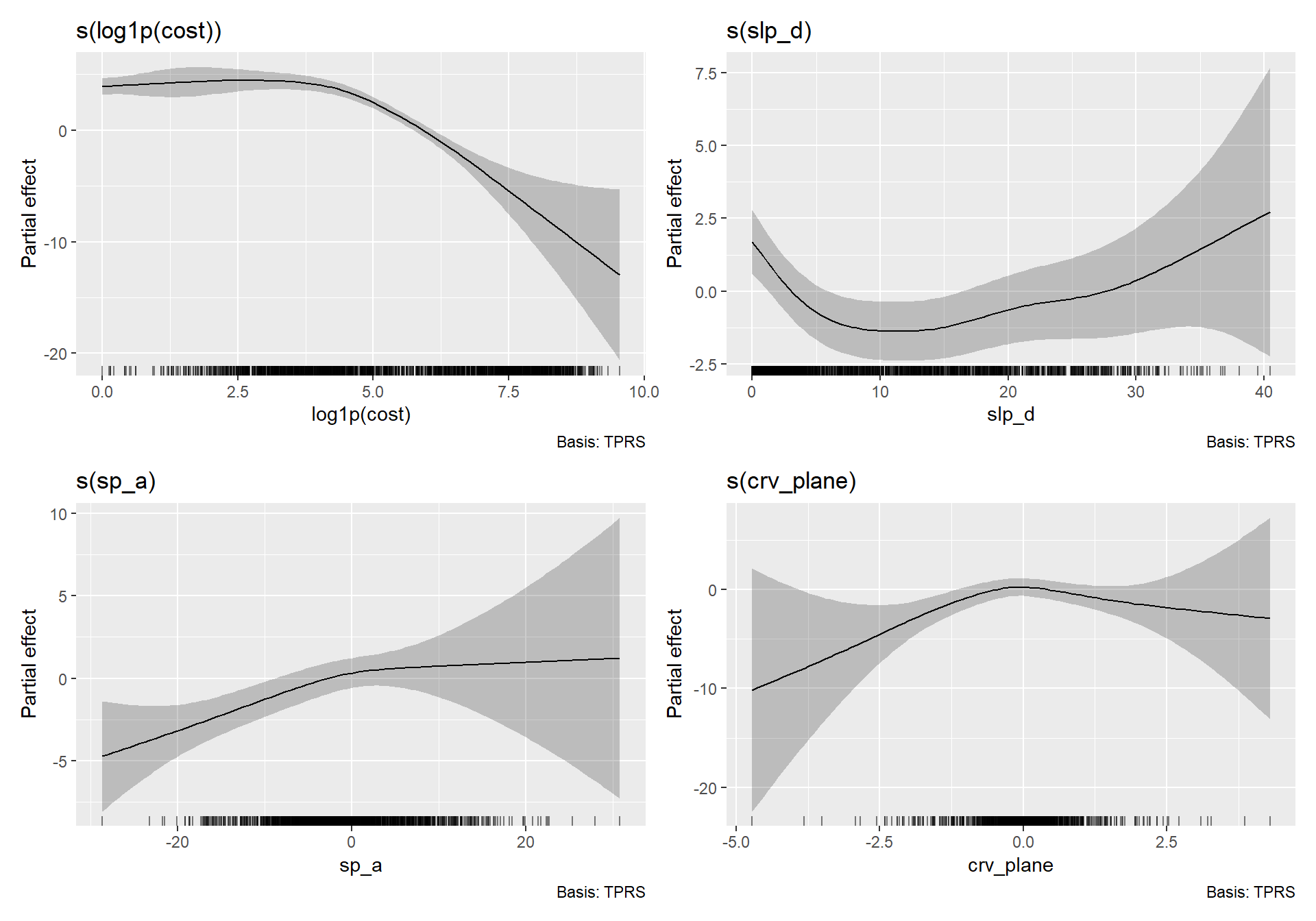
The shape functions can be interpreted as follows:
- Cost (log scale): The contribution is high and nearly constant for locations close to water bodies, then decreases steeply once the log-transformed cost exceeds about 4.5 (a cost of roughly 90). Locations far from water are very unlikely to be wetlands.
- Slope: The likelihood of being a wetland is highest on flat terrain and decreases rapidly as slope increases up to about 10 degrees. Beyond that, the curve rises slightly, but the confidence interval becomes very wide since few training samples occur on steep slopes. This part of the curve should not be over-interpreted.
- Slope position: Wetlands are less likely in locations that are much lower than their surroundings (large negative values), with the contribution increasing up to a slope position near 0. Above 0, the curve flattens and the confidence interval widens substantially.
- Plan curvature: The contribution peaks near 0 and decreases for strongly convergent (negative) locations, although the confidence interval is wide at the extremes.
Note that the confidence intervals widen wherever training data are sparse. This is valuable information that is not readily available from most machine learning models: it tells us where the model is uncertain about the relationship.
The partial effects are on the log-odds scale, which is additive. Exponentiating a difference in partial effects gives an odds ratio. For example, if the partial effect of slope decreases by 2 between two slope values, then the odds of being a wetland are \(e^{-2} \approx 0.14\) times as large at the steeper slope, holding the other variables constant.
11.4.4 Comparison to Logistic Regression
Since a logistic regression model is a GAM with linear shape functions, it is informative to compare the two. We fit a logistic regression model with the same predictor variables using glm(). In the logistic regression model, slope position is not statistically significant. However, in the GAM, it is highly significant. The relationship is non-linear and non-monotonic, so a straight line does not capture it. The Akaike information criterion (AIC), which balances model fit and complexity, is substantially lower for the GAM, which indicates a better model.
                Estimate Std. Error      z value     Pr(>|z|)
(Intercept)  5.769469945 0.33417244  17.26494847 8.638091e-67
log1p(cost) -0.806783015 0.06703096 -12.03597507 2.299016e-33
slp_d       -0.305218783 0.02284787 -13.35874177 1.053295e-40
sp_a         0.001334904 0.02135638   0.06250609 9.501598e-01
crv_plane 0.971976375 0.16802745 5.78462835 7.267282e-09AIC(glmM, gamM) df AIC
glmM 5.00000 857.8923
gamM 17.85042 587.868611.4.5 Explaining Individual Predictions
Since a GAM is additive, the prediction for any location can be decomposed into the contribution of each term. Setting type = "terms" in predict() returns the contribution of each smooth, and the constant attribute provides the intercept. Below, we explain the predictions for two validation samples: one wetland and one upland. Summing the intercept and the term contributions gives the predicted log-odds, which are converted to a probability with plogis().
sites <- test[c(1, 1001), ]
sites
# A tibble: 2 × 5
class cost slp_d sp_a crv_plane
<fct> <dbl> <dbl> <dbl> <dbl>
1 Wetland 0 0.114 -4.50 0
2 Upland 3458. 14.7 -9.64 -0.268| intercept | log_odds | probability | class | s(log1p(cost)) | s(slp_d) | s(sp_a) | s(crv_plane) |
|---|---|---|---|---|---|---|---|
| −1.350 | 4.164 | 0.985 | Wetland | 3.916 | 1.630 | −0.272 | 0.241 |
| −1.350 | −11.460 | 0.000 | Upland | −7.828 | −1.256 | −1.200 | 0.175 |
For the wetland sample, which is located directly adjacent to water on flat terrain, the large positive contributions from cost and slope result in a predicted probability near 1. For the upland sample, which is far from water on a moderately steep slope, the large negative contribution from cost dominates, resulting in a probability near 0. This type of exact, local explanation is only an approximation for black-box models, such as random forest, but is inherent to additive models.
11.4.6 Model Checking
There are two common checks for GAMs. First, k.check() assesses whether the basis dimension, k, is large enough. If the edf is close to k' (the maximum possible edf), the smooth may be too constrained, and k should be increased. Here, all edfs are well below 9. The k-index is less than 1 with a small p-value for the cost smooth, which suggests some remaining pattern in the residuals. However, refitting the model with k = 20 for cost barely changes the edf or the AIC, so the basis dimension is adequate. For binary responses, the k-index should be interpreted cautiously.
k.check(gamM) k' edf k-index p-value
s(log1p(cost)) 9 4.086924 0.8653389 0.00
s(slp_d) 9 4.392074 0.9527069 0.03
s(sp_a) 9 2.316257 0.9594377 0.05
s(crv_plane) 9 3.347818 0.9589713 0.05 df AIC
gamM 17.85042 587.8686
gamK20 18.08076 588.0304Second, concurvity() assesses concurvity, the non-linear analogue of collinearity. It measures the degree to which each smooth can be approximated by the other smooths in the model, with values ranging from 0 to 1. High concurvity makes the shape functions unstable and difficult to interpret, since the model cannot separate the effects of the related variables. The “estimate” row is generally the most useful. The cost and slope smooths have moderate concurvity (around 0.5 to 0.6), which is consistent with their correlation, while slope position and plan curvature are relatively independent of the other terms. This is why we limited the model to four predictor variables that represent different terrain characteristics. If we had included several variables that measure similar characteristics, such as slope and roughness, their shape functions would be much harder to interpret.
concurvity(gamM, full = TRUE) |> round(2) para s(log1p(cost)) s(slp_d) s(sp_a) s(crv_plane)
worst 0 0.82 0.79 0.54 0.25
observed 0 0.81 0.54 0.39 0.14
estimate 0 0.62 0.53 0.33 0.1011.5 Explainable Boosting Machines
11.5.1 Train the Model
EBMs are trained using ebm_classify() from interpret. Unlike mgcv, this function does not use a formula. Instead, it requires a data frame of predictor variables (X) and a numeric vector of class labels coded as 0 and 1 (y). We code wetlands as 1. Since EBMs bin the predictor variables and learn step functions, they are not affected by monotonic transformations, so we use the original “cost” values.
Key arguments of ebm_classify() include the following. We use the default settings.
-
max_bins: the maximum number of bins used to discretize each predictor variable (default of 255) -
outer_bags: the number of bagged models that are averaged (default of 16) -
learning_rate: the boosting learning rate (default of 0.01) -
max_leaves: the maximum number of leaves in each tree (default of 3) -
validation_size,early_stopping_rounds, andmax_rounds: a portion of the training data is withheld to determine when to stop boosting
trainX <- train |> select(all_of(predsToUse)) |> as.data.frame()
trainY <- as.integer(train$class == "Wetland")
testX <- test |> select(all_of(predsToUse)) |> as.data.frame()

ebmM <- ebm_classify(trainX, trainY)
The model is stored as two lists: cuts, which contains the bin boundaries for each predictor variable, and term_scores, which contains the score for each bin. Together, these define the step-like shape functions. Making a prediction simply involves looking up the score for each predictor variable, summing the scores, and converting the sum to a probability.
In our testing of version 0.1.35 of the interpret package, the term scores returned by ebm_classify() were shrunk by a factor equal to the number of outer bags. As a result, the predicted probabilities were compressed toward 0.5: the ranking of the predictions, and therefore the AUC ROC, was correct, but the probabilities were poorly calibrated. Training with outer_bags = 1 produced scores approximately 16 times larger than the default of 16 bags. We correct for this by multiplying the term scores by the number of outer bags. If you are using a different version of the package, check whether this correction is still needed by examining the range of the predicted probabilities before and after applying it.
range(ebm_predict_proba(ebmM, testX))[1] 0.3546081 0.5725635nBags <- 16
ebmM$term_scores <- lapply(ebmM$term_scores, \(s) s * nBags)
range(ebm_predict_proba(ebmM, testX))[1] 6.898767e-05 9.907797e-0111.5.2 Shape Functions
The ebm_show() function plots the shape function for a single predictor variable. As with the GAM, the y-axis represents the contribution, or score, on the log-odds scale. Below, we plot the shape function for each predictor variable.
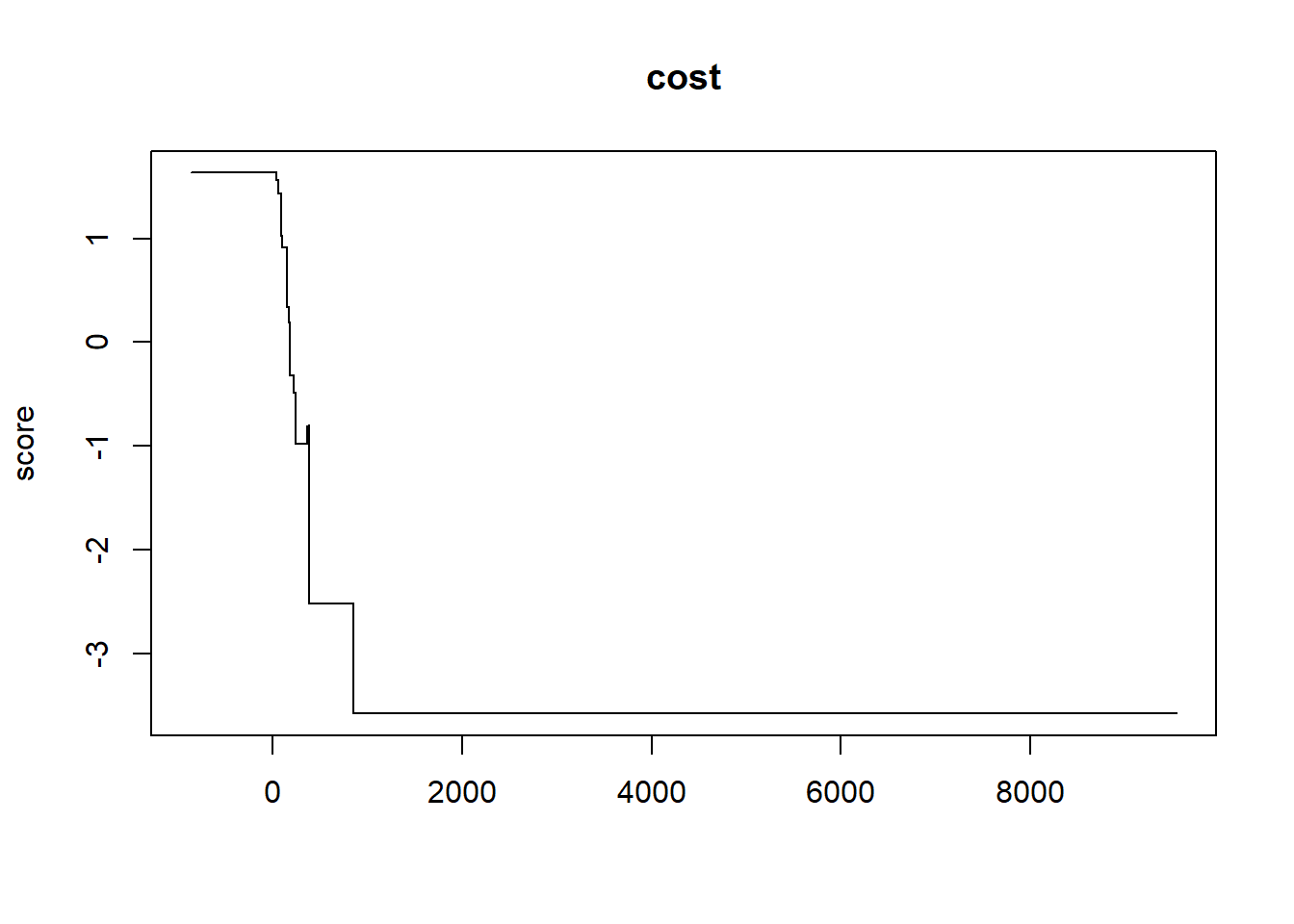
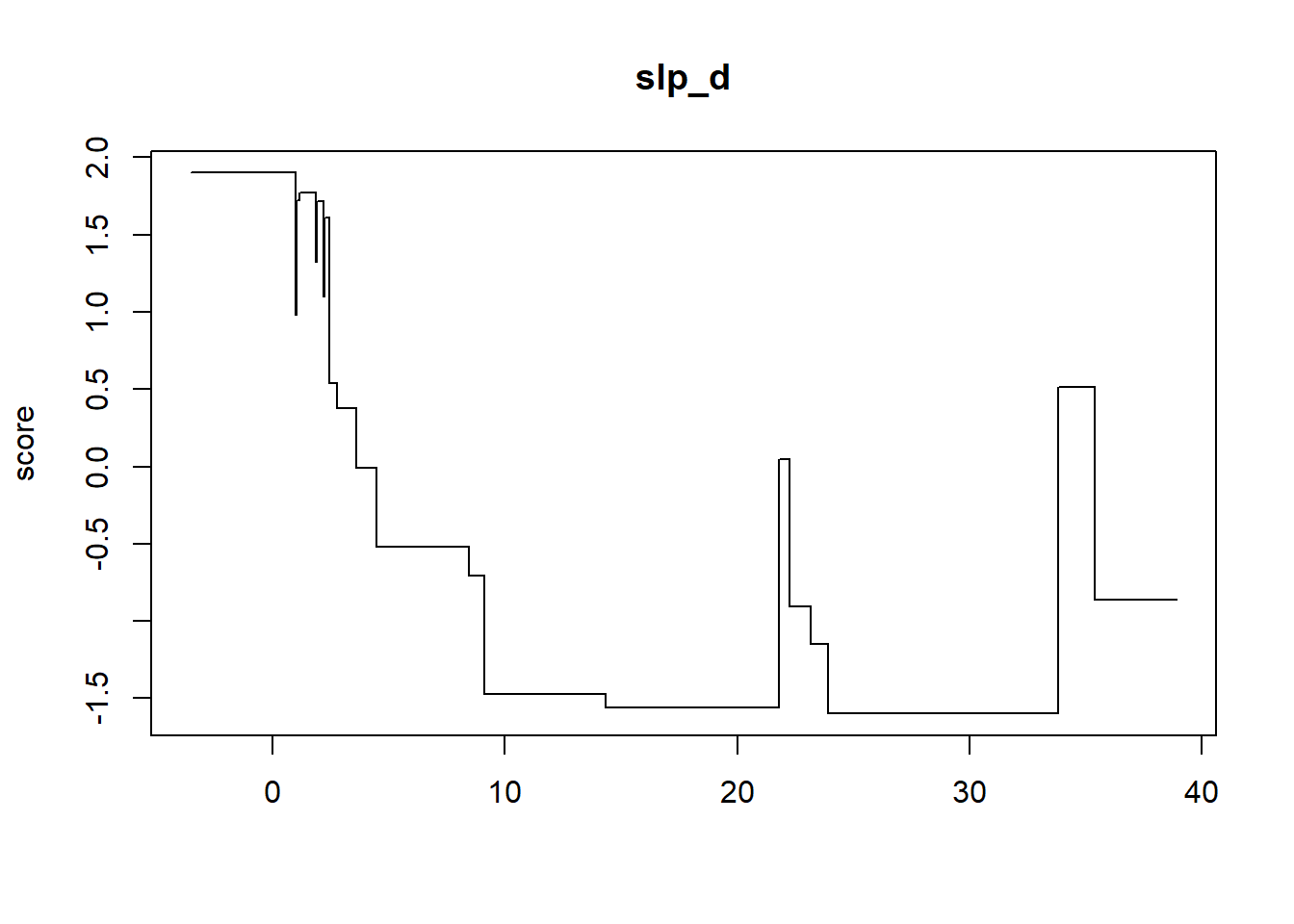
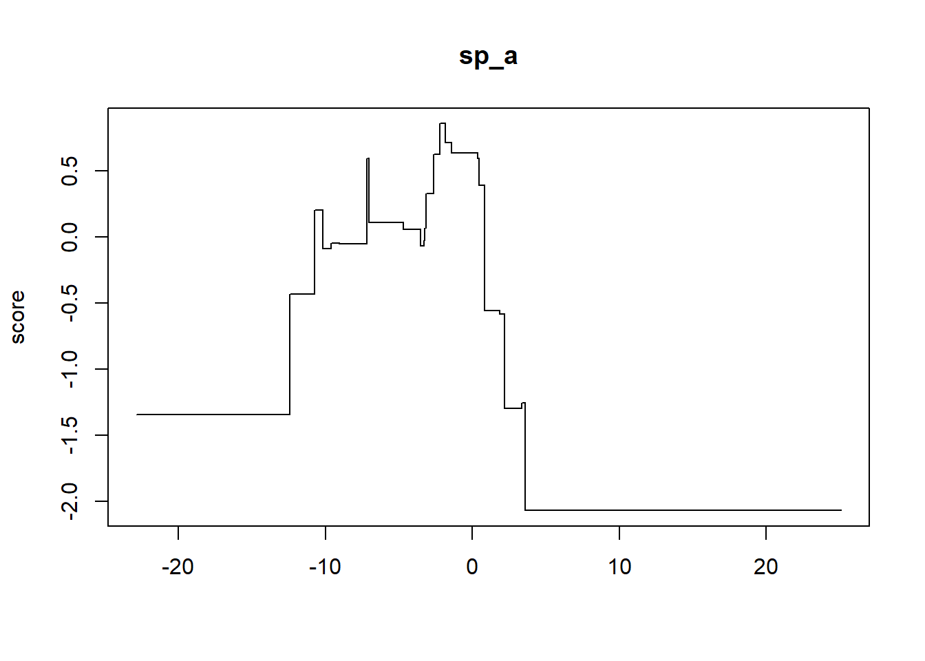
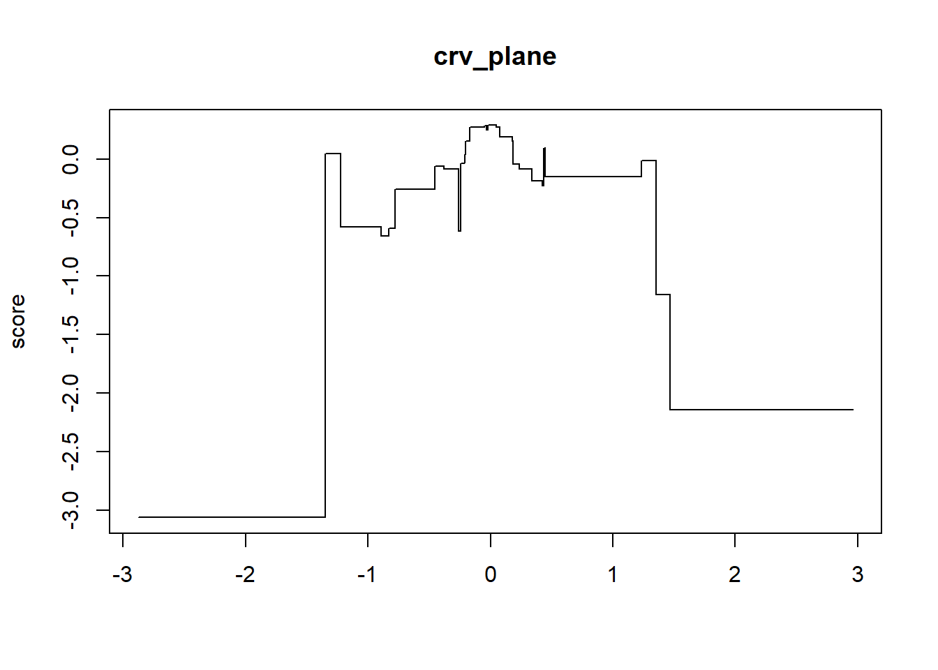
The EBM shape functions are step functions as opposed to smooth curves. The cost shape function shows that the score is high near water and decreases sharply between costs of roughly 50 and 900, after which it is flat. Since the EBM uses the original values, this abrupt decrease occurs over a small portion of the x-axis. The slope shape function decreases rapidly from flat terrain up to about 9 degrees, similar to the GAM, and is then mostly flat, apart from a few narrow spikes at steeper slopes where there are few training samples. The slope position shape function peaks for locations near 0 and decreases for both low and high positions, and the plan curvature shape function is highest near 0.
Note that the EBM shape functions extend as flat lines beyond the range of most of the training data. Unlike the GAM, the EBM does not provide confidence intervals, so it does not indicate where the shape function is poorly supported by the data.
11.5.3 Explaining Individual Predictions
Since ebm_predict_proba() only returns probabilities, we write a short function to obtain the contribution of each predictor variable for a set of samples. For each predictor variable, findInterval() identifies the bin in which each value falls, and the corresponding score is extracted. The first element of each set of term scores is reserved for missing values, so we offset the bin index by 2. We confirm that summing the contributions and converting to a probability reproduces the output of ebm_predict_proba().
ebmTerms <- function(model, data) {
  map(names(model$cuts), \(v) {
    binIdx <- findInterval(data[[v]], model$cuts[[v]])
    model$term_scores[[v]][binIdx + 2]
  }) |>
    set_names(names(model$cuts)) |>
    as_tibble()
}

testTerms <- ebmTerms(ebmM, testX)
max(abs(plogis(rowSums(testTerms)) - ebm_predict_proba(ebmM, testX)))
[1] 2.220446e-16We now explain the predictions for the same two validation samples used above. The EBM has no separate intercept, so the sum of the contributions is the predicted log-odds. As with the GAM, cost provides the largest contribution for both samples.
ebmTerms(ebmM, as.data.frame(sites)) |>
  mutate(log_odds = rowSums(across(everything())),
         probability = plogis(log_odds),
         class = sites$class, .before = 1) |>
  gt() |>
fmt_number(decimals = 3)| log_odds | probability | class | cost | slp_d | sp_a | crv_plane |
|---|---|---|---|---|---|---|
| 3.880 | 0.980 | Wetland | 1.634 | 1.901 | 0.058 | 0.288 |
| −5.318 | 0.005 | Upland | −3.578 | −1.560 | −0.091 | −0.088 |
11.5.4 Variable Importance
For an additive model, a natural measure of global variable importance is the mean absolute contribution of each predictor variable across the training samples. This is the measure used by the InterpretML library. Unlike the permutation-based measures discussed in Chapter 10, it is calculated directly from the model. Cost is the most important predictor variable, followed by slope, slope position, and plan curvature.
ebmImp <- ebmTerms(ebmM, trainX) |>
  summarize(across(everything(), \(s) mean(abs(s)))) |>
  pivot_longer(everything(), names_to = "variable", values_to = "importance")

ggplot(ebmImp, aes(x = importance, y = reorder(variable, importance))) +
  geom_col(fill = "#B03A2E") +
  labs(x = "Mean Absolute Score", y = "Predictor Variable") +
  theme_bw()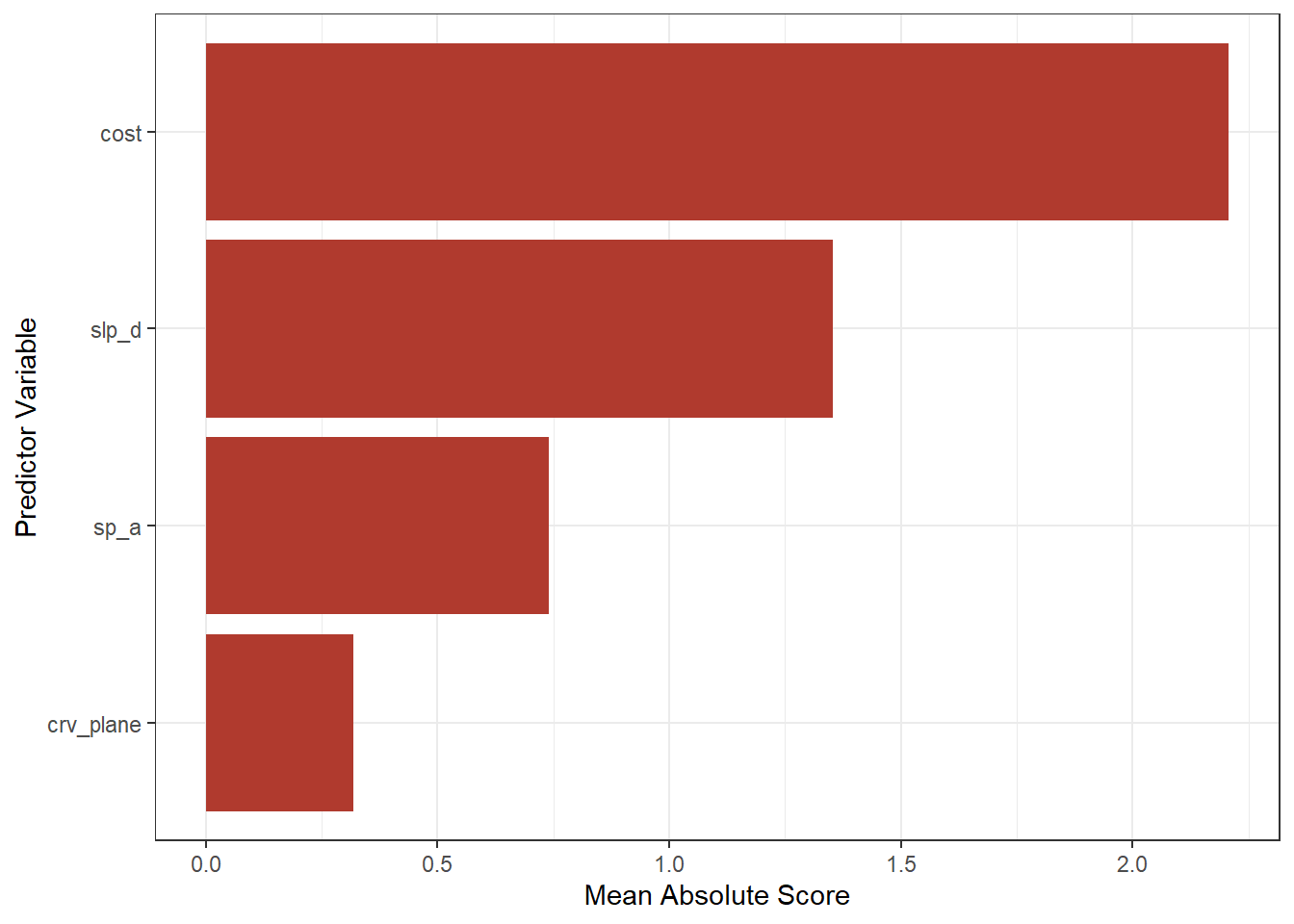
11.6 Comparing the Models
11.6.1 Shape Functions
Since both models have the same additive structure, we can directly compare their shape functions. For each predictor variable, we create a sequence of values between the 1st and 99th percentiles of the training data, which avoids the sparse tails. The GAM contributions are obtained with predict(type = "terms"). The other predictor variables are set to their medians, but this does not affect the contribution of the variable of interest since the model is additive. The EBM contributions are obtained with our ebmTerms() function. Since the two models center their shape functions differently, we center each shape function on its mean contribution across the training data so that they can be compared.
gamTrainTerms <- predict(gamM, train, type = "terms")
ebmTrainTerms <- ebmTerms(ebmM, trainX)

shapeCompare <- map(seq_along(predsToUse), \(i) {
  v <- predsToUse[i]
  newD <- train |>
    summarize(across(all_of(predsToUse), median)) |>
    slice(rep(1, 200))
  newD[[v]] <- seq(quantile(train[[v]], 0.01),
                   quantile(train[[v]], 0.99),
                   length.out = 200)
  tibble(variable = v,
         value = newD[[v]],
         GAM = predict(gamM, newD, type = "terms")[, i] - mean(gamTrainTerms[, i]),
         EBM = ebmTerms(ebmM, as.data.frame(newD))[[v]] - mean(ebmTrainTerms[[v]]))
}) |>
  bind_rows() |>
  pivot_longer(c(GAM, EBM), names_to = "model", values_to = "contribution")

ggplot(shapeCompare, aes(x = value, y = contribution, color = model)) +
  geom_line(linewidth = 1) +
  facet_wrap(~variable, scales = "free") +
  scale_color_manual(values = c("EBM" = "#DBAF5A", "GAM" = "#B03A2E")) +
  labs(x = "Predictor Variable Value", y = "Contribution (log-odds)", color = "Model") +
  theme_bw()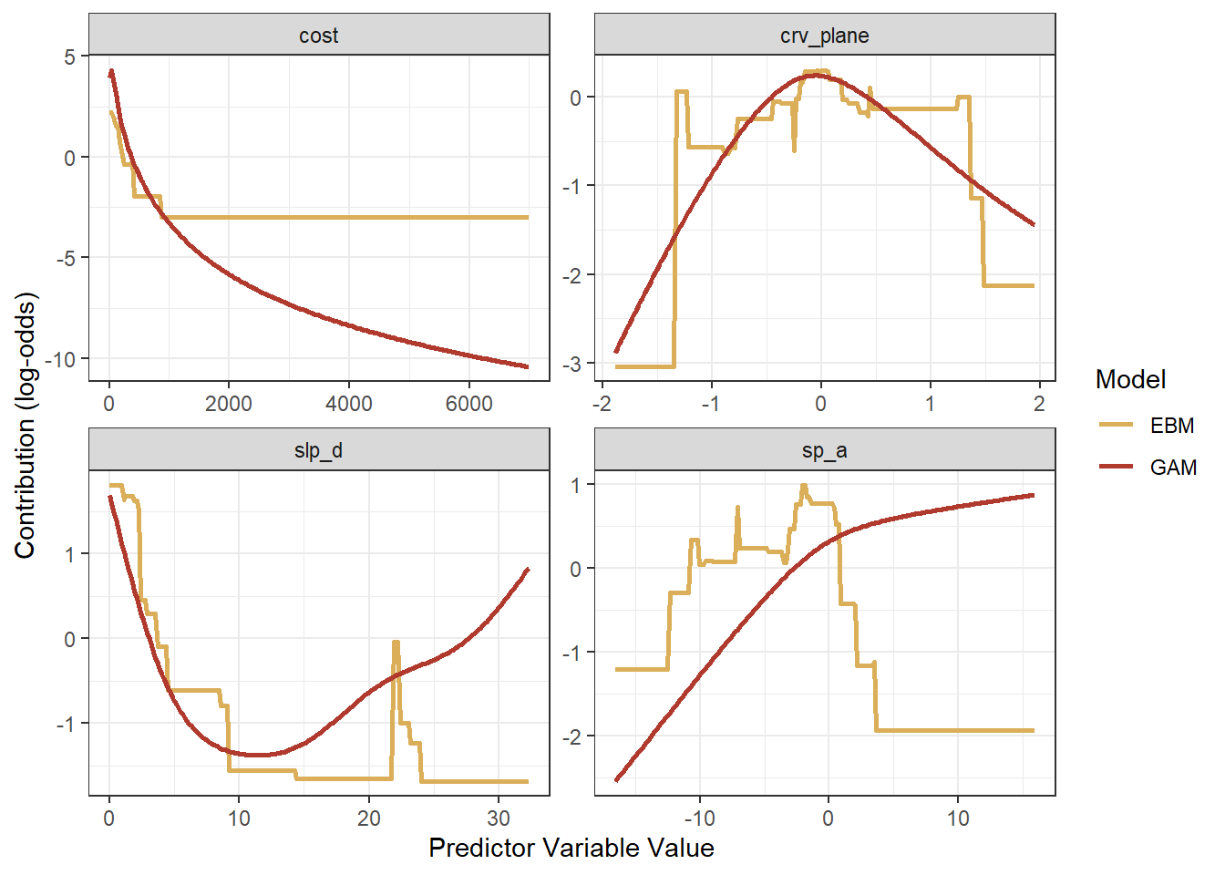
The two models agree where most of the training data occur: both assign high contributions to locations close to water, on gentle slopes, and with plan curvature near 0. However, they diverge elsewhere:
- Cost: Both decrease rapidly over the first several hundred units. Beyond that, the EBM shape function is flat, while the GAM continues to decrease since the smooth was fit on the log scale and extends the trend.
- Slope: Both decrease up to about 10 degrees. Above about 12 degrees, the GAM curve increases while the EBM shape function remains low.
- Slope position: The models disagree the most. The GAM increases steadily, while the EBM peaks just below 0 and then drops for higher slope positions.
- Plan curvature: Both peak near 0, but the EBM drops abruptly at the extremes, while the GAM decreases gradually.
In each case, the disagreement occurs where training data are sparse, which is also where the GAM’s confidence intervals are widest. In these ranges, the data do not strongly constrain the shape function, so the result depends on the assumptions of each model: the GAM’s penalty favors smooth curves that extend existing trends, while the EBM’s binning favors flat steps. This highlights an important point: interpretable models show us exactly what the model learned, but what a model learned is not necessarily the true relationship, especially where data are sparse. Comparing multiple interpretable models and considering uncertainty are good practices.
11.6.2 Predictive Performance
Interpretability is only useful if the model also performs well. Below, we calculate the AUC ROC, overall accuracy (using a 0.5 threshold), and log loss for the GAM, EBM, and logistic regression models using the validation data. Both additive models substantially outperform logistic regression. Their AUC ROC values are also close to those of the tuned random forest models in Chapter 16 (approximately 0.988), even though those models used eight predictor variables as opposed to four.
testProbs <- tibble(class = test$class,
                    GAM = predict(gamM, test, type = "response"),
                    EBM = ebm_predict_proba(ebmM, testX),
                    Logistic = predict(glmM, test, type = "response"))

testProbs |>
  pivot_longer(-class, names_to = "model", values_to = "prob") |>
  group_by(model) |>
  summarize(roc_auc = roc_auc_vec(class, prob, event_level = "second"),
            accuracy = mean((prob > 0.5) == (class == "Wetland")),
            log_loss = mn_log_loss_vec(class, prob, event_level = "second")) |>
  arrange(desc(roc_auc)) |>
  gt() |>
fmt_number(decimals = 4)| model | roc_auc | accuracy | log_loss |
|---|---|---|---|
| GAM | 0.9861 | 0.9440 | 0.1449 |
| EBM | 0.9848 | 0.9470 | 0.1499 |
| Logistic | 0.9676 | 0.9405 | 0.2084 |
11.7 Predict to Raster Data
Lastly, we use both models to predict to raster data. As in Chapter 10, we read in the predictor variable stack and the forest mask. We do not need to transform the “cost” raster since the log transformation is part of the GAM formula. To reduce processing time, we predict to a 600 by 600 cell subset of the full extent.
predStk <- rast(str_glue("{fldPth}predictors.tif"))

names(predStk) <- c("cost", "crv_arc", "crv_plane", "crv_pro", "ctmi",
                    "diss_5", "diss_10", "diss_20", "diss_25", "diss_a",
                    "rough_5", "rough_10", "rough_20", "rough_25", "rough_a",
                    "slp_d", "sp_5", "sp_10", "sp_20", "sp_25", "sp_a")

predSub <- predStk[[predsToUse]][601:1200, 601:1200, drop = FALSE]

forMsk <- rast(str_glue("{fldPth}for_mask.tif"))
predSub <- mask(predSub, crop(forMsk, predSub))
For the GAM, predict() from terra can pass the type = "response" argument directly to the mgcv prediction function. For the EBM, we provide a short function that converts each block of raster values to a data frame and calls ebm_predict_proba(). The two predictions are combined into a single raster stack for mapping.
gamMap <- predict(predSub, gamM, type = "response", na.rm = TRUE)

ebmMap <- predict(predSub, ebmM,
                  fun = \(model, data, ...) ebm_predict_proba(model, as.data.frame(data)),
                  na.rm = TRUE)

probMaps <- c(gamMap, ebmMap)
names(probMaps) <- c("GAM", "EBM")tm_shape(probMaps) +
tm_raster(col.scale = tm_scale_continuous(values = "brewer.yl_gn_bu"),
col.legend = tm_legend(title = "Wetland Probability"),
col.free = FALSE) +
tm_facets_wrap(ncol = 2)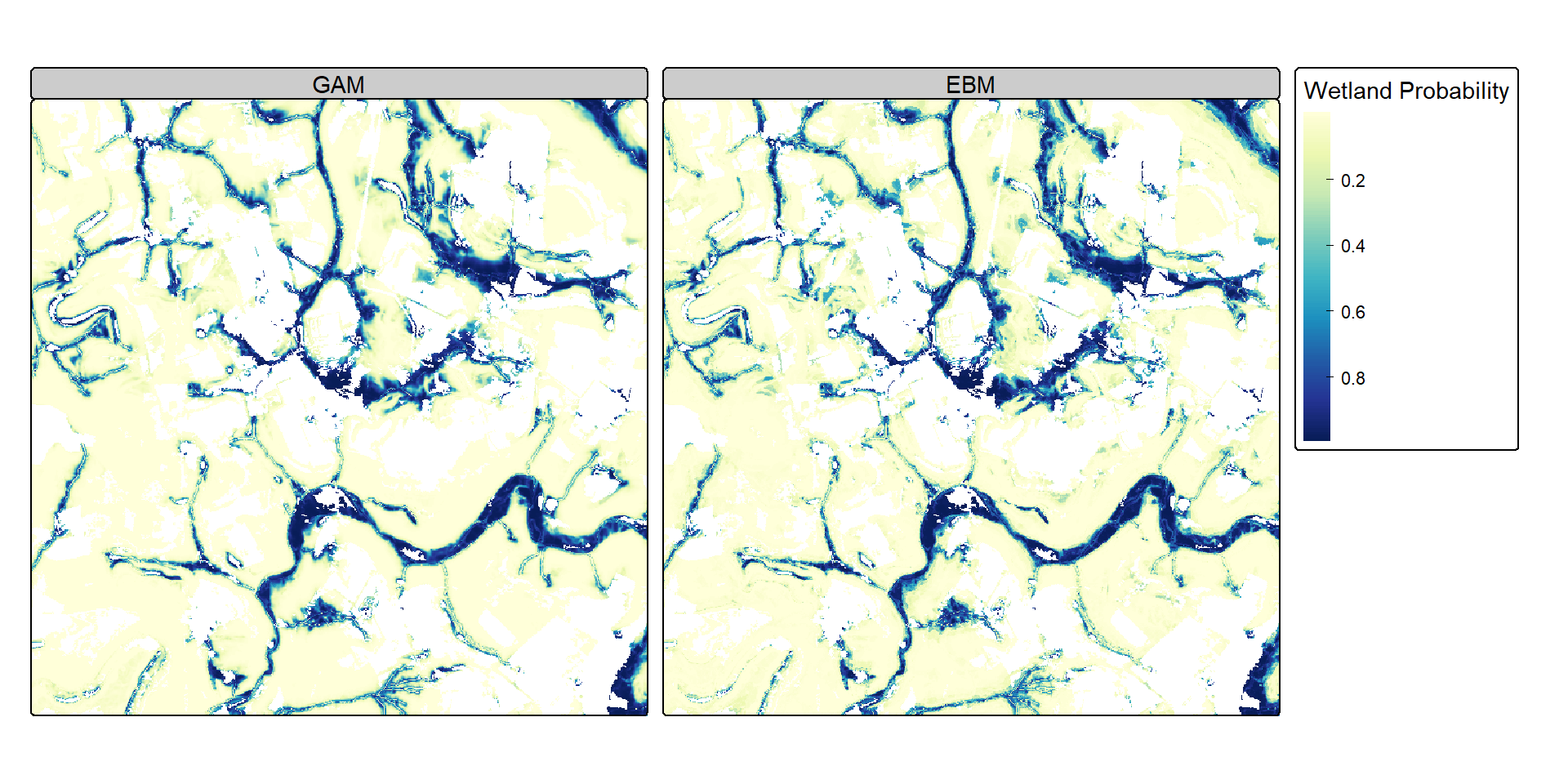
The two maps show very similar patterns, with high wetland probabilities along valley bottoms adjacent to streams. The EBM map shows slightly sharper transitions between low and high probabilities, which reflects its step-like shape functions.
11.8 Concluding Remarks
In this chapter, we explored two interpretable alternatives to black-box machine learning models. GAMs and EBMs both model the response as a sum of shape functions, each of which depends on a single predictor variable. As a result, the shape functions fully describe the model, and every prediction can be decomposed exactly into the contributions of the predictor variables. GAMs, as implemented in mgcv, produce smooth shape functions with confidence intervals and can be used for a wide variety of response types. EBMs, as implemented in interpret, learn step-like shape functions using boosting and can capture abrupt changes. For the wetland mapping problem, both models performed nearly as well as random forest models that used twice as many predictor variables, while being much easier to interpret.
The main limitation of additive models is that they do not automatically model interactions between predictor variables. Interactions can be added to GAMs using tensor product smooths, such as te(slp_d, sp_a), and to EBMs using pairwise interaction terms in the Python version of InterpretML, but each interaction term makes the model somewhat harder to interpret. Also, as with any model, interpretable models show what the model learned from the data, which may not reflect the true underlying relationships where data are sparse or predictor variables are strongly related.
11.9 Questions
- Explain the difference between an interpretable (“glass-box”) model and a post hoc explanation of a black-box model.
- Explain how logistic regression is a special case of a GAM.
- What does the effective degrees of freedom (edf) of a smooth term represent?
- What is the role of the penalty in a GAM, and how is its strength determined when using
method = "REML"? - Explain how an EBM learns its shape functions.
- Why does a monotonic transformation, such as the log transformation, change the GAM but not the EBM?
- What is concurvity, and why does it make shape functions difficult to interpret?
- Explain how the prediction for a single location can be decomposed into the contributions of each predictor variable for an additive model.
- Why might the shape functions learned by a GAM and an EBM disagree?
11.10 Exercises
In these exercises, you will apply GAMs and EBMs to the landslide susceptibility problem introduced in the Chapter 10 exercises. The goal is to model the likelihood of landslide occurrence within the Valley and Ridge physiographic province of West Virginia using topographic predictor variables and to interpret the learned relationships. You have been provided with the following files in the exercise folder for the chapter.
- chpt11.gpkg/lsPnts: point locations representing landslide locations and pseudo-absence locations where predictor variables have been extracted
- stk.tif: raster stack of predictor variables for a portion of the study area
The following digital terrain model (DTM) derived land surface parameter (LSP) predictor variables have been provided. Other than elevation, the LSPs were calculated at three different window sizes, indicated by the numbers 1 through 3.
- “elev”: elevation in meters
- “slp1”/“slp2”/“slp3”: topographic slope in degrees
- “sar1”/“sar2”/“sar3”: surface area ratio (SAR)
- “tri1”/“tri2”/“tri3”: topographic roughness index (TRI)
- “tpi1”/“tpi2”/“tpi3”: topographic position index (TPI)
- “diss1”/“diss2”/“diss3”: topographic dissection index
The “class” column differentiates landslides (“slpF”) from pseudo-absence samples (“not”).
Data Preparation
Task 1
- Read in the lsPnts layer, drop the geometry information, and drop the “elev” column.
- Convert the “class” column to a factor with levels
c("not", "slpF")so that the models predict the probability of the second level, landslide occurrence. - Use
initial_split()from rsample to randomly split the data into equal-sized training and test sets, stratified by class. Set a random seed so that your results are reproducible. - Read in the raster stack and rename the bands to match the predictor variable columns in the table, including “elev”. The bands are in the same order as the columns.
- Calculate the correlation matrix for all predictor variables. Which variables are highly correlated with each other? Why does this matter when building and interpreting additive models?
Generalized Additive Model
Task 2
- Using the training data, fit a logistic GAM with mgcv that includes smooths of slope (“slp1”), topographic position (“tpi1”), and dissection (“diss2”). Use
method = "REML". - Interpret the model summary. Are all smooths statistically significant? Based on the effective degrees of freedom, which relationships are the most non-linear?
- Use
gratia::draw()to plot the shape functions. Describe the relationship between each predictor variable and the likelihood of landslide occurrence. Where are the confidence intervals widest, and why? - Use
k.check()andconcurvity()to check the model. - Fit a logistic regression model with the same three predictor variables using
glm()and compare it to the GAM using AIC. Does allowing non-linear relationships improve the model?
Task 3
- Add a smooth of the topographic roughness index (“tri1”) to the GAM from Task 2.
- Use
concurvity()to assess the new model andgratia::draw()to plot its shape functions. - How did the slope shape function and its confidence interval change when roughness was added? Explain this result in terms of the correlation between slope and roughness. What does this suggest about selecting predictor variables for interpretable models?
Explainable Boosting Machine
Task 4
- Train an EBM using
ebm_classify()from interpret with the same three predictor variables used in Task 2. Code landslides as 1 and pseudo-absences as 0. - Check whether the term score correction described in this chapter is needed for your version of interpret by comparing the range of the predicted probabilities before and after multiplying the term scores by the number of outer bags. Apply the correction if needed.
- Use
ebm_show()to plot the shape function for each predictor variable. - Calculate the mean absolute score of each predictor variable across the training samples. Which variable is the most important?
- Following the approach used in this chapter, plot the GAM and EBM shape functions for each predictor variable on the same axes. Where do the two models agree, and where do they disagree? Do the disagreements occur where data are sparse?
Assess and Map
Task 5
- Use the test set to calculate the AUC ROC, overall accuracy (using a 0.5 threshold), and log loss for the GAM, EBM, and logistic regression models. Which model performed best?
- Choose two test samples, one landslide and one pseudo-absence, and decompose the predictions of the GAM and EBM into the contributions of each predictor variable. Which variable contributes most to each prediction?
- Use the GAM and EBM to predict the probability of landslide occurrence to a 1,000 by 1,000 cell subset of the raster stack. Map both predictions using tmap and describe the spatial patterns.
- Compare your results to the random forest model from the Chapter 10 exercises. Do the interpretable models achieve similar performance? What do you gain, and what do you lose, by using an interpretable model in place of random forest for this problem?