13 Improving Deep Learning Models
13.1 Topics Discussed
- Implementing drop-outs
- Implementing batch normalization
- Using different activation functions
- Increasing the receptive field of convolutional layers using atrous or dilated convolution
- Implementing and parameterizing alternative loss functions (weighted cross entropy (CE), focal binary cross entropy (BCE)/focal CE, Dice, Tversky, and focal Tversky)
- Using and parameterizing optimizers (mini-batch stochastic gradient descent (SGD), adaptive gradient (adagrad), root mean square propagation (RMSprop), and adaptive moment estimation (Adam)
- Selecting learning rates and using the learning rate finder process
- Implementing weight decay and momentum
- Using schedulers during the training loop
- Using learning rate schedulers
13.2 Introduction
A wide variety of techniques have been developed to potentially improve the accuracy of deep learning (DL) models. Before moving on to semantic segmentation problems, we will explore some commonly used methods. It should be noted that new methods and techniques are being developed since this is an active area of research. Here, we focus on some widely used methods. We also discuss some methods specific to semantic segmentation in the remaining chapters of this section.
We have organized this discussion into methods that relate to modifying the model architecture, loss function modifications or alternatives to traditional binary cross entropy (BCE) or cross entropy (CE), optimizer selection and configuration, and training process modifications.
The methods discussed generally attempt to combat common issues or complexity, such as overfitting and reduced generalization. Some method also focus on allowing models to be successfully trained using a smaller set of training samples. Lastly, other methods attempt to reduce the impact of class imbalance.
We do not train any models in this chapter. Instead, we provides code snippets that can be used within complete training workflows.
13.3 Model Architecture Changes
13.3.1 Dropout
Dropouts are a regularization method in which certain neurons are dropped out or their associated parameters are not updated within the training loop during passes over training mini-batches. The idea is that not updating all of the weights/parameters during each weight update can result in reduced overfitting and improved generalization. How many neurons will be dropped in each weight update is controlled by the p parameter. In the example model architecture below, we are applying dropouts between each fully connected layer, which will cause a random 30% of the neurons to not be updated with each weight/parameter update. Note that we do not use dropouts after the final fully connected layer. Dropouts are implemented using nn_dropout() from torch.
Dropouts can be used after fully connected layers and also after convolutional layers. For convolutional layers, individual weights within kernels can be dropped or entire feature maps. Generally, dropout rates are higher for fully connected layers in comparison to convolutional layers.
There is currently some debate as to whether dropouts are still necessary. With the advent and wide adoption of batch normalization, dropouts have generally been used less frequently. Analysts are using batch normalization as a means to potentially reduce overfitting and improve generalization as opposed to dropouts, and including both dropouts and batch normalization may be unnecessary. Again, analysts and researchers have varying opinions. We generally prefer to use batch normalization as opposed to dropouts. However, you may want to experiment with dropouts as a potential means to improve model performance.
The example CNN architecture below implements dropouts after the second convolutional layer and after the fully connected layer.
cnnModelDO <- nn_module(

  "SimpleCNNwithDO",

  initialize = function(input_channels = 3,
                        num_classes = 10,
                        dropout_rate = 0.5){

    self$conv1 <- nn_conv2d(input_channels, 32,
                            kernel_size = 3,
                            padding = 1)

    self$conv2 <- nn_conv2d(32,
                            64,
                            kernel_size = 3,
                            padding = 1)

    self$pool <- nn_max_pool2d(kernel_size = 2,
                               stride = 2)

    self$drop1 <- nn_dropout(p = dropout_rate)

    self$fc1 <- nn_linear(64 * 8 * 8, 128)

    self$drop2 <- nn_dropout(p = dropout_rate)

    self$output <- nn_linear(128, num_classes)

  },

  forward = function(x) {

    x <- nnf_relu(self$conv1(x))
    x <- self$pool(x)

    x <- nnf_relu(self$conv2(x))
    x <- self$pool(x)

    x <- self$drop1(x)

    x <- x$view(c(x$size(1), -1))

    x <- nnf_relu(self$fc1(x))
    x <- self$drop2(x)

    x <- self$output(x)

    return(x)
  }
)
13.3.2 Batch Normalization
You have already seen examples of batch normalization in the last two chapters. In modern architectures, it is common to include batch normalization after fully connected layers and convolutional layers and before applying an activation function. In torch, batch normalization is applied using nn_batch_norm1d() or nn_batch_norm2d(). Using the output of a fully connected layer as an example, batch normalization is applied by first calculating the mean and variance of each activation from the prior fully connected layer separately for all the samples in the mini-batch then using these measurements to convert the activations to z-scores. The data can then be further augmented using scale and shift parameters, which are trainable. For convolutional layers, batch normalization is performed separately for each learned feature map per mini-batch and requires calculating separate means and variances for each feature map using their associated kernel weights. Separate trainable scale and shift parameters can then be applied to each feature map.
Although batch normalization has been empirically documented to improve model performance, the reason for the improvement is still debated. The originators of the method suggest that including these layers helps minimize the issue of covariate shift. Later studies suggest that the improvement results from allowing training processes to bypass local minima and allowing for training using larger learning rates, which can speed up the training process. It has also been suggested that it smooths the optimization landscape, which makes it easier to apply meaningful parameter updates. Others have suggested that it behaves as a form of regularization. Regardless of the reason, we have generally found batch normalization to be useful and generally suggest including it throughout DL architectures. We generally prefer to use batch normalization as opposed to dropouts, and some have argued that dropouts are not necessary or less helpful when using batch normalization.
As you have already seen in the prior modules, the code below shows how to apply batch normalization. nn_batch_norm1d() is used after fully connected layers while nn_batch_norm2d() is used after convolutional layers. Activation functions are generally applied after batch normalization is applied. The number of added trainable parameters for 1D batch normalization is equal to 2 times the number of input activations, since each activation has an associated shift and scale parameter. For 2D batch normalization, the number of trainable parameters is equal to 2 times the number of output feature maps from the prior layer.
cnnModelBN <- nn_module(

  "CNNWithBatchNorm",

  initialize = function(input_channels = 3,
                        num_classes = 10){

    self$conv1 <- nn_conv2d(input_channels,
                            32,
                            kernel_size = 3,
                            padding = 1)

    self$bn1 <- nn_batch_norm2d(32)

    self$conv2 <- nn_conv2d(32,
                            64,
                            kernel_size = 3,
                            padding = 1)

    self$bn2 <- nn_batch_norm2d(64)

    self$pool <- nn_max_pool2d(kernel_size = 2,
                               stride = 2)

    self$fc1 <- nn_linear(64 * 8 * 8, 128)

    self$bn3 <- nn_batch_norm1d(128)

    self$output <- nn_linear(128, num_classes)
  },

  forward = function(x) {

    x <- self$conv1(x)
    x <- self$bn1(x)
    x <- nnf_relu(x)
    x <- self$pool(x)

    x <- self$conv2(x)
    x <- self$bn2(x)
    x <- nnf_relu(x)
    x <- self$pool(x)

    x <- x$view(c(x$size(1), -1))

    x <- self$fc1(x)
    x <- self$bn3(x)
    x <- nnf_relu(x)

    x <- self$output(x)

    return(x)

  }
)
13.3.3 Alternative Activation Functions
There are alternative activation functions that can be used in place of the rectified linear unit (ReLU) function. One issue with ReLU is the “dying ReLU” problem where all activations approach zero. This results in a very low gradient and difficulty updating the model parameters using backpropagation and an optimization algorithm. One alternative is leaky ReLU where the negative activations are not converted to zero. Instead, the negative activations are maintained but at a reduced magnitude by multiplying them by a positive value smaller than 1 (for example, 0.01). This negative slope term is defined by the user. Alternatively, parameterized ReLU allows the negative slope term to be trainable during the learning process. As another example, a swish activation consists of multiply the activation by the activation passed through a sigmoid function. There are other activation functions, these are just a few commonly used examples.
The example model below allows the user to select between the three activation functions just described using the added act_fn parameter. If leaky ReLU is used, the user can also specify the negative slope term.
Although there are multiple opinions regarding alternative activation functions, we have generally found that using leaky ReLU or swish in place of ReLU rarely results in decreased performance. However, the change may not greatly impact model performance in all cases. As a result, we often using leaky ReLU by default and in place of ReLU. However, this is just our opinion.
cnnModelBNAct <- nn_module(

  "CNNWithBatchNormAndActivation",

  initialize = function(input_channels = 3,
                        num_classes = 10,
                        act_fn = "relu",
                        negative_slope = 0.01
  ){

    self$conv1 <- nn_conv2d(input_channels,
                            32, kernel_size = 3,
                            padding = 1)

    self$bn1 <- nn_batch_norm2d(32)

    self$conv2 <- nn_conv2d(32,
                            64,
                            kernel_size = 3,
                            padding = 1)

    self$bn2 <- nn_batch_norm2d(64)

    self$pool <- nn_max_pool2d(kernel_size = 2,
                               stride = 2)

    self$fc1 <- nn_linear(64 * 8 * 8, 128)

    self$bn3 <- nn_batch_norm1d(128)

    self$output <- nn_linear(128,
                             num_classes)

    self$act_fn_name <- act_fn

    self$negative_slope <- negative_slope

    if(act_fn == "prelu") {

      self$prelu <- nn_prelu(num_parameters = 1)
    }
  },

  apply_activation = function(x) {

    if(self$act_fn_name == "relu") {

      return(nnf_relu(x))

    } else if(self$act_fn_name == "leaky_relu") {

      return(nnf_leaky_relu(x,
                            negative_slope=self$negative_slope))

    } else if(self$act_fn_name == "prelu") {

      return(self$prelu(x))

    } else if (self$act_fn_name == "swish") {

      return(x * x$sigmoid())

    } else {

      stop(paste0("Unsupported activation function: ",
                  self$act_fn_name))

    }
  },

  forward = function(x) {

    x <- self$conv1(x)
    x <- self$bn1(x)
    x <- self$apply_activation(x)
    x <- self$pool(x)

    x <- self$conv2(x)
    x <- self$bn2(x)
    x <- self$apply_activation(x)
    x <- self$pool(x)

    x <- x$view(c(x$size(1), -1))

    x <- self$fc1(x)
    x <- self$bn3(x)
    x <- self$apply_activation(x)

    x <- self$output(x)

    return(x)

  }
)
13.3.4 Dilated Convolution
One potential drawback of convolutional layers in comparison to some more modern architectures, such as those based on transformers or mamba, is the small size of the receptive field. Since it is common to use small moving windows, such as 3x3, 5x5, or 7x7, only local context is captured. In order to capture larger scale context, pooling operations, such as max pooling, are often applied in order to increase the receptive field while still using small kernel sizes. However, this requires decreasing the spatial detail of the input data. One option would be to just use larger kernel sizes; however, this greatly increases the number of trainable weights in the kernel and the computational complexity of the model.
One means to increase the receptive field without increasing the number of weights or trainable parameters is to use atrous or dilated convolution. Essentially, zeros are placed inside of the kernel so that non-adjacent cells can be used in the convolution operation.
The word atrous is derived from the French term “à trous” meaning”with holes.”
In order to implement atrous or dilated convolution, a dilation argument must be provided within nn_conv2d(). Be default, this is set to 1 so that no zeros are added to the kernel and directly adjacent cells are considered. If dilation = 3, this means that 2 zeros will be placed between the center cell and the cells considered in the convolution operation. In order to maintain the number of rows and columns of cells in the output, the padding parameter should be equal to the dilation rate and the stride should be 1. If a kernel size other than 3x3 is used, dilation will be added between all cells used. For example, for a 5x5 kernel with a dilation rate of 4, 3 cells would be placed between the center cell and the first set of cells followed by 3 zeros between the first set and last set of cells.
Dilated convolution is a core component of some architectures, such as the DeepLab-family. It is also used in specific modules, such as the atrous spatial pyramid pooling (ASPP) module, which will be discussed in the context of semantic segmentation architectures later in this section of the text.
The architecture below demonstrates how to implement dilated convolution. The user is able to set the dilation rate separately for the two convolutional layers used in the architecture.
cnnModelBNDilated <- nn_module(
  "CNNWithBatchNormAndDilation",

  initialize = function(input_channels = 3,
                        num_classes = 10,
                        dilation1 = 1,
                        dilation2 = 1){

    self$conv1 <- nn_conv2d(
      in_channels = input_channels,
      out_channels = 32,
      kernel_size = 3,
      padding = dilation1,
      dilation = dilation1
    )

    self$bn1 <- nn_batch_norm2d(32)

    self$conv2 <- nn_conv2d(
      in_channels = 32,
      out_channels = 64,
      kernel_size = 3,
      padding = dilation2,
      dilation = dilation2
    )

    self$bn2 <- nn_batch_norm2d(64)

    self$pool <- nn_max_pool2d(kernel_size = 2,
                               stride = 2)

    self$fc1 <- nn_linear(64 * 8 * 8, 128)

    self$bn3 <- nn_batch_norm1d(128)

    self$output <- nn_linear(128,
                             num_classes)

  },

  forward = function(x) {

    x <- self$conv1(x)
    x <- self$bn1(x)
    x <- nnf_relu(x)
    x <- self$pool(x)

    x <- self$conv2(x)
    x <- self$bn2(x)
    x <- nnf_relu(x)
    x <- self$pool(x)

    x <- x$view(c(x$size(1), -1))

    x <- self$fc1(x)
    x <- self$bn3(x)
    x <- nnf_relu(x)

    x <- self$output(x)

    return(x)

  }
)
13.4 Alternative Loss Functions
There are some shortcoming of the traditional binary cross entropy (BCE) and cross entropy (CE) losses. The equations for these losses are provided below. For BCE loss, the user is not able to specify the relative weighting of the background and presence classes, and, for CE loss, the user is not able to specify the relative weighting of each class in the combined metric. Since each sample contributes equally, the more abundant class(es) will have a higher weight in the classification. This can result in the modeling doing a poorer job predicting less abundant classes or over-predicting the occurrence of the more abundant classes. Another issue is that these methods do not allow the user to place additional weight on difficult-to-predict samples. Thus, there is a need for alternative loss metrics or means to augment BCE or CE loss.
\[ \mathcal{L}_{\text{BCE}} = - \left[ y \cdot \log(\hat{p}) + (1 - y) \cdot \log(1 - \hat{p}) \right] \]
\[ \mathcal{L}_{\text{CE}} = - \sum_{c=1}^{C} y_c \cdot \log(\hat{p}_c) \]
13.4.1 Class Weightings
CE loss, as implemented with nn_cross_entropy_loss(), allows for specifying relative class weightings via the weight parameter. The argument for this parameter should be a 1D tensor of weights equal in length to the number of classes. In our example, we first generate an R vector then convert it to a torch tensor with a float data type. This tensor is then used when instantiating an instance of CE loss.
\[ \mathcal{L}_{\text{weighted-CE}} = - \sum_{c=1}^{C} \alpha_c \cdot y_c \cdot \log(\hat{p}_c) \]
In order for classes to take on equal weightings, their weights can be defined relative to the inverse of the abundance of the class in the training set. This will cause samples from the less abundant classes to have a higher weight in the aggregated loss relative to samples from the more abundant classes. The user could also choose to place disproportionately more weight on specific classes, perhaps if these classes are most important for the task at hand.
class_weights <- c(0.2, 0.3, 0.5)

weight_tensor <- torch_tensor(class_weights,
                              dtype = torch_float())

weighted_ce_loss <- nn_cross_entropy_loss(weight = weight_tensor)
13.4.2 Focal Loss
Focal losses allow for placing more weight on more difficult samples, which are defined as samples that have a low predicted logit or class probability for their correct assignment. Practically, this results in the model being penalized more for misclassifying difficult samples.
The code block below provides example implementations of focal BCE and focal CE loss. A custom implementation is necessary since torch does not provide these losses natively. The key parameter is gamma. Larger values of gamma result in increased weight being applied to difficult samples. For focal BCE loss, alpha controls the relative weight of the background and foreground classes. For focal CE loss, it controls the relative weight of each class.
\[ \mathcal{L}_{\text{focal-BCE}}(y, \hat{p}) = - \alpha \cdot y \cdot (1 - \hat{p})^{\gamma} \cdot \log(\hat{p}) - (1 - \alpha) \cdot (1 - y) \cdot \hat{p}^{\gamma} \cdot \log(1 - \hat{p}) \]
\[ \mathcal{L}_{\text{focal-CE}} = - \sum_{c=1}^C \alpha_c \cdot \delta_{c=y} \cdot (1 - \hat{p}_c)^{\gamma} \cdot \log(\hat{p}_c) \]
focal_bce_loss <- function(pred,
                           target,
                           alpha = 0.25,
                           gamma = 2.0,
                           reduction = "mean",
                           epsilon = 1e-6) {

  # Convert logits to probabilities using sigmoid function
  pred_prob <- pred$sigmoid()

  # Make sure target and predictions have the same data type
  target <- target$to(dtype = pred_prob$dtype)

  # Calculate focal correction factor
  pt <- pred_prob * target + (1 - pred_prob) * (1 - target)

  # Apply alpha
  alpha_t <- alpha * target + (1 - alpha) * (1 - target)

  # Calculate per-sample loss
  loss <- -alpha_t * (1 - pt)$pow(gamma) * (pt + epsilon)$log()

  # Aggregate loss
  if(reduction == "mean"){

    return(loss$mean())

  } else if(reduction == "sum"){

    return(loss$sum())

  } else{

    return(loss)

  }
}

focal_ce_loss <- function(pred,
                          target,
                          alpha = NULL,
                          gamma = 2.0,
                          reduction = "mean",
                          epsilon = 1e-6) {

  # Get number of classes
  num_classes <- pred$size(2)

  # Convert from logits to probabilities using a soft max function
  pred_prob <- pred$softmax(dim = 2)

  # Convert target codes to one-hot encoding
  target_onehot <- torch_nn_functional_one_hot(target$long(),
                                               num_classes)$permute(c(1, 4, 2, 3))$to(dtype = pred$dtype)

  # Get pt: predicted probability of the true class
  pt <- (pred_prob * target_onehot)$sum(dim = 2)  # [B, H, W]

  # Class weights
  if (!is.null(alpha)) {

    # alpha is a numeric vector of length C (one weight per class)
    alpha_tensor <- torch_tensor(alpha,
                                 dtype = pred$dtype,
                                 device = pred$device)

    alpha_t <- (target_onehot * alpha_tensor$view(c(1, -1, 1, 1)))$sum(dim = 2)

  } else {

    alpha_t <- torch_ones_like(pt)

  }

  # Per-sample focal loss
  loss <- -alpha_t * (1 - pt)$pow(gamma) * (pt + epsilon)$log()

  # Aggregate loss
  if (reduction == "mean") {

    return(loss$mean())

  } else if (reduction == "sum") {

    return(loss$sum())

  } else {

    return(loss)

  }
}
13.4.3 Dice and Tversky
BCE and CE loss, and their weighted and focal derivatives, are generally termed distribution-based losses. There are also region-based losses that make use of true positive (TP), false positive (FP), and false negative (FN) predicted probabilities. Probabilities are used, as opposed to counts, in order to make the loss differentiable.
The Dice loss is generally the most commonly used region-based loss. Ignoring the use of probabilities as opposed to hard counts, it is equivalent to 1 minus the Dice coefficient. The Dice coefficient is equivalent to the F1-score assessment metric discussed in Chapter 5. For a multiclass problem, macro-averaging is used to aggregate the class-level losses. In other words, the loss is calculated separately for each class then averaged such that each class has equal weight in the aggregated loss. This is one of the main reasons that the Dice loss can be useful in cases of class imbalance, and this is especially true in cases of extreme class imbalance. For example, in mapping tasks it is common for the class of interest to make up a small proportion of the landscape being mapped and the associated training set. We have generally found the Dice loss to be particularly useful for semantic segmentation tasks with extreme class imbalance, as will be demonstrated in the later chapters of this section.
\[ \mathcal{L}_{\text{Dice}} = 1 - \frac{2 \cdot \text{TP}}{2 \cdot \text{TP} + \text{FP} + \text{FN}} \]
\[ \mathcal{L}_{\text{Dice}} = 1 - \frac{1}{C} \sum_{c=1}^{C} \frac{2 \cdot \text{TP}_c}{2 \cdot \text{TP}_c + \text{FP}_c + \text{FN}_c} \]
The Tversky loss is a modification of the Dice loss that allows the user to control the relative weighting of FP and FN errors, as specified using alpha and beta terms, respectively. For a multiclass problem, as with the multiclass Dice loss, the loss is calculated separately for each class then aggregated using macro averaging. It is also possible to use different alpha and beta terms for each class and to apply different weightings for each class in the final aggregation.
\[ \mathcal{L}_{\text{Tversky}} = 1 - \frac{\text{TP}}{\text{TP} + \alpha \cdot \text{FP} + \beta \cdot \text{FN}} \]
\[ \mathcal{L}_{\text{Tversky}} = 1 - \frac{1}{C} \sum_{c=1}^{C} \frac{\text{TP}_c}{\text{TP}_c + \alpha \cdot \text{FP}_c + \beta \cdot \text{FN}_c} \]
The code blocks below show implementations of the binary Dice and Tversky losses (first code block) and multiclass Dice and Tversky losses (second code block). We also demonstrate a multiclass focal Tversky loss, which, similar to the focal version of CE loss, allows for placing more weight on difficult-to-predict classes.
dice_loss <- function(pred,
                      target,
                      epsilon = 1e-6) {

  # Convert logits to probabilities using sigmoid function
  pred <- pred$sigmoid()

  # Flatten
  pred_flat <- pred$view(c(-1))
  target_flat <- target$view(c(-1))

  # Calcualte numerator
  intersection <- (pred_flat * target_flat)$sum()

  # Calculate denominator
  union <- pred_flat$sum() + target_flat$sum()

  # Calculate loss
  loss <- 1 - ((2 * intersection + epsilon) / (union + epsilon))

  return(loss)

}


tversky_loss <- function(pred,
                         target,
                         alpha = 0.5,
                         beta = 0.5,
                         epsilon = 1e-6) {

  # Convert logits to probabilities using sigmoid function
  pred <- pred$sigmoid()

  # Flatten
  pred_flat <- pred$view(c(-1))
  target_flat <- target$view(c(-1))

  # Calculate components
  TP <- (pred_flat * target_flat)$sum()
  FP <- (pred_flat * (1 - target_flat))$sum()
  FN <- ((1 - pred_flat) * target_flat)$sum()

  # Calculate loss
  tversky <- (TP + epsilon) / (TP + alpha * FP + beta * FN + epsilon)
  loss <- 1 - tversky

  return(loss)

}
dice_loss_multiclass <- function(pred,
target,
epsilon = 1e-6) {
# pred: [B, C, H, W] — raw logits
# target: [B, H, W] — integer class labels
# Get number of classes
num_classes <- pred$size(2)
# Convert logits to probabilties using a softmax function
pred <- pred$softmax(dim = 2)
# Convert class targe class indices to one-hot encoding
target_onehot <- torch_nn_functional_one_hot(target$long(),
num_classes = num_classes)$permute(c(1, 4, 2, 3))$to(dtype = pred$dtype)
# Flatten per class
pred_flat <- pred$reshape(c(pred$size(1), pred$size(2), -1))
target_flat <- target_onehot$reshape(c(target_onehot$size(1), target_onehot$size(2), -1))
#Calculate numerator
intersection <- (pred_flat * target_flat)$sum(dim = 3)
#Calculate denominator
union <- pred_flat$sum(dim = 3) + target_flat$sum(dim = 3)
#Calculate loss
dice_score <- (2 * intersection + epsilon) / (union + epsilon)
dice_loss <- 1 - dice_score$mean()
return(dice_loss)
}
tversky_loss_multiclass <- function(pred,
target,
alpha = 0.5,
beta = 0.5,
epsilon = 1e-6) {
# pred: [B, C, H, W]
# target: [B, H, W]
#Get number of classes
num_classes <- pred$size(2)
# Convert logits to class probabilties using softmax function
pred <- pred$softmax(dim = 2)
# Convert target class indices to one-hot encoding
target_onehot <- torch_nn_functional_one_hot(target$long(), num_classes = num_classes)$permute(c(1, 4, 2, 3))$to(dtype = pred$dtype)
# Flatten
pred_flat <- pred$reshape(c(pred$size(1), pred$size(2), -1))
target_flat <- target_onehot$reshape(c(target_onehot$size(1), target_onehot$size(2), -1))
# Calculate components
TP <- (pred_flat * target_flat)$sum(dim = 3)
FP <- (pred_flat * (1 - target_flat))$sum(dim = 3)
FN <- ((1 - pred_flat) * target_flat)$sum(dim = 3)
#Calculate loss
tversky_index <- (TP + epsilon) / (TP + alpha * FP + beta * FN + epsilon)
tversky_loss <- 1 - tversky_index$mean()
return(tversky_loss)
}focal_tversky_loss_multiclass <- function(pred,
target,
alpha = 0.5,
beta = 0.5,
gamma = 1.33,
epsilon = 1e-6) {
# pred: [B, C, H, W] - raw logits
# target: [B, H, W] - class indices
# Get number of classes
num_classes <- pred$size(2)
# Convert logits to probabilities using softmax function
pred <- pred$softmax(dim = 2)
# Convert target class indices to one-hot encoding
target_onehot <- torch_nn_functional_one_hot(target$long(), num_classes = num_classes)$permute(c(1, 4, 2, 3))$to(dtype = pred$dtype)
# Flatten
pred_flat <- pred$reshape(c(pred$size(1), pred$size(2), -1))
target_flat <- target_onehot$reshape(c(target_onehot$size(1), target_onehot$size(2), -1))
#Calculate components
TP <- (pred_flat * target_flat)$sum(dim = 3)
FP <- (pred_flat * (1 - target_flat))$sum(dim = 3)
FN <- ((1 - pred_flat) * target_flat)$sum(dim = 3)
#Calculate loss
tversky_index <- (TP + epsilon) / (TP + alpha * FP + beta * FN + epsilon)
focal_tversky <- (1 - tversky_index)$pow(gamma)
loss <- focal_tversky$mean()
return(loss)
}13.5 Optimizers
There are a variety of different optimization algorithms made available by torch including mini-batch stochastic gradient descent (SGD) (optim_sgd()), adaptive gradient (adagrad) (optim_adagrad()), root mean square propagation (RMSprop) (optim_rmsprop()), and adaptive moment estimation (adam) (optim_adam()). Example instantiations of different optimizers are shown in the following code block. We generally use adam as our default optimizer, but others may disagree.
optimizer_sgd <- optim_sgd(
  params = model$parameters,
  lr = 0.01,
  momentum = 0.9,
  weight_decay = 1e-4
)

optimizer_rmsprop <- optim_rmsprop(
  params = model$parameters,
  lr = 0.01,
  alpha = 0.99,
  weight_decay = 1e-4
)

optimizer_adamw <- optim_adamw(
  params = model$parameters,
  lr = 0.001,
  weight_decay = 1e-2
)
13.5.1 Optimizer Options
There are additional options that can be specified for optimization algorithms. Generally, the learning rate is considered to be the most important setting. Higher learning rates yield larger weight updates with each optimization step. However, if the learning rate is too large, gradient explosion and unstable learning can occur. If the learning rate is too small, the learning process can progress slowly and/or the model may get stuck in a local minimum.
13.5.2 Learning Rate Finder
A method was proposed to select an appropriate learning rate or range of learning rates in the following paper:
Smith, L.N., 2017, March. Cyclical learning rates for training neural networks. In 2017 IEEE winter conference on applications of computer vision (WACV) (pp. 464-472). IEEE.
The learning rate finder procedure has been implemented in luz. Once a fitted luz model object has been created, the lr_finder() function can be used to implement this process. The model will train for an epoch beginning with the lowest learning rate. With each mini-batch and associated optimization step, the learning rate increases. Initially, the loss will likely not improve, since the learning rate is too low to allow for meaningful weight updates. Once the learning rate increases to the point where meaningful updates can be made, the loss will start to decrease. Eventually, the learning rate will become too large, gradient explosion will occur, and the loss will increase. Generally, the optimal learning rates are those associated with the region of decreasing loss. The learning rate at the lowest loss is generally not considered the best since this is close to when gradient explosion occurs. The results of this test can be noisy; however, it offers some guidance on the optimal learning rate or range of learning rates to consider. We generally suggest that this is worth implementing.
We have implemented the learning rate finder process using luz in the following code blocks and for the problem explored in Chapter 11. In the first block we (1) set the folder path, (2) load the training data table, (3) prepare the training data using dplyr and recipes, (4) define a custom torch dataset subclass, (5) instantiate an instance of the dataset subclass for the training set, (6) instantiate the training dataloader, and (7) define the fully connected model architecture by subclassing nn_module(). In the second code block, we instantiate the luz fitted object. Finally, we run the learning rate finder process then graph the results. We specifically test values between 1e-6 and 1.
If you want to run this example, you will need to use the data provided with Chapter 11. The required data were not replicated into the Chapter 13 folder.
The results generally suggest a learning rate ~1e-3 is a good choice. This learning rate occurs within the region of decreasing loss. 1e-1 would be too high even though it is near the lowest loss since it is close to where gradient explosion begins or the loss begins to increase.
It is important to run the learning rate finder process using the same settings that will be used to train the model. For example, you would want to use the same optimization algorithm and mini-batch size. This is because changes to these settings can impact the optimal learning rate.
library(tidyverse)
library(recipes)
library(yardstick)

fldPth <- "gslrData/chpt11/data/"

euroSatTrain <- read_csv(str_glue("{fldPth}train_aggregated.csv")) |>
  mutate_if(is.character, as.factor) |>
  select(-1) |>
  mutate(code = code+1) |>
  sample_frac(1, replace=FALSE)

myRecipe <- recipe(class ~ ., data = euroSatTrain) |>
  step_range(all_numeric_predictors(), -c(code),
             min=0,
             max=1,
             clipping=FALSE)

myRecipePrep <- prep(myRecipe, training=euroSatTrain)

trainProcessed <- bake(myRecipePrep, new_data=NULL)

tabDataset <- torch::dataset(

  name = "tabDataSet",

  initialize = function(df){
    self$df <- df
  },

  .getitem = function(i){

    preds <- self$df[i, 2:11] |>
      unlist() |>
      as.vector() |>
      unname()
    label <- self$df[i, 12] |>
      unlist() |>
      as.numeric() |>
      as.vector() |>
      unname()

    predsT <- preds |>
      torch_tensor(dtype=torch_float32())

    labelT <- label |>
      torch_tensor(dtype=torch_int64())
    labelT <- labelT$squeeze()

    return(list(preds = predsT, label = labelT))
  },

  .length = function(){

    return(nrow(self$df))

  }
)

trainDS <- tabDataset(trainProcessed)

trainDL <- torch::dataloader(trainDS,
                             batch_size=120,
                             shuffle=TRUE,
                             drop_last = TRUE)


myANN <- torch::nn_module(
  "ANN",

  initialize = function(inFeat=10,
                        nNodes=c(32,64,128),
                        nCls) {

    self$inFeat = inFeat
    self$nNodes = nNodes
    self$nCls = nCls

    self$net <- nn_sequential(
      nn_linear(inFeat, nNodes[1]),
      nn_batch_norm1d(nNodes[1]),
      nn_relu(),
      nn_linear(nNodes[1], nNodes[2]),
      nn_batch_norm1d(nNodes[2]),
      nn_relu(),
      nn_linear(nNodes[2], nNodes[3]),
      nn_batch_norm1d(nNodes[3]),
      nn_relu(),
      nn_linear(nNodes[3], nCls)
    )

  },

  forward = function(x) {

    x <- self$net(x)
    return(x)

  }
)
model <- myANN |>
setup(
loss = nn_cross_entropy_loss(),
optimizer = optim_adam
) |>
set_hparams(
inFeat=10,
nNodes=c(32,64,128),
nCls=10
) lr_result <- lr_finder(object = model,
data = trainDL,
start_lr = 1e-6,
end_lr = 1)plot(lr_result)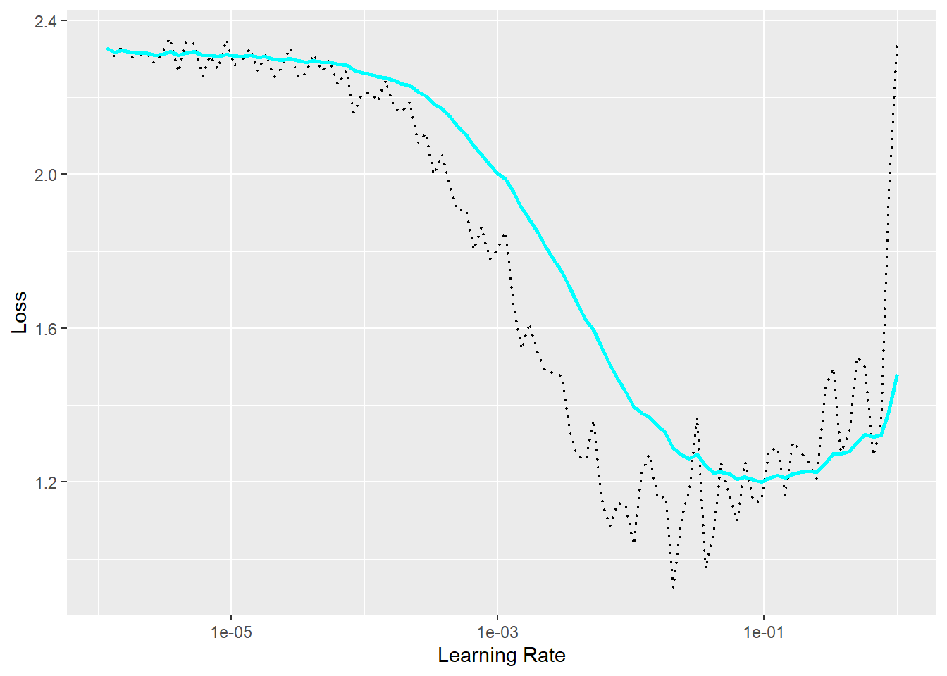
13.5.3 Weight Decay
Weight decay is a form of L2 regularization which shrinks the magnitude of the weight updates as the model progresses in an attempt to reduce overfitting. It is implemented by adding a penalty to the loss function that increases as the magnitudes of the model parameters increase. This is similar to the regularization applied when using ridge regression. Within torch optimizers, weight decay is controlled by the weight_decay parameter. If weight decay is used with adam, it is recommended to use the optim_adamw() version of the optimizer since weight decay is not implemented correctly in the original version of adam. If no weight decays is used, optim_adam() and optim_adamw() are equivalent.
# Dummy model
model <- nn_module(
  initialize = function() {
    self$fc <- nn_linear(10, 1)
  },
  forward = function(x) {
    self$fc(x)
  }
)

# Instantiate model
net <- model()

# Define SGD optimizer with momentum and weight decay
optimizer <- optim_sgd(
  params = net$parameters,
  lr = 0.01,              # learning rate
  weight_decay = 0.0005   # L2 regularization (weight decay)
)
13.5.4 Momentum
Momentum encourages the optimizer to continue to proceed in the same direction in the loss space relative to prior parameter updates. This is generally accomplished by considering prior updates as opposed to only the current gradient for each optimization step. Momentum can be incorporated with optim_sgd() using the momentum parameter. Note that adam is essentially RMSprop with momentum added.
# Dummy model
model <- nn_module(
  initialize = function() {
    self$fc <- nn_linear(10, 1)
  },
  forward = function(x) {
    self$fc(x)
  }
)

# Instantiate model
net <- model()

# Define SGD optimizer with momentum and weight decay
optimizer <- optim_sgd(
  params = net$parameters,
  lr = 0.01,              # learning rate
  momentum = 0.9,         # momentum term
)
13.6 Training Process Modifications
In this final section, we provide some example methods for augmenting the training process to potentially improve performance or model generalization.
13.6.1 Callbacks
Callbacks are used to offer conditional control or allow for modifying the training loop at different steps or locations within the loop. For example, callbacks can be implemented at the end of each epoch, after each optimization step, if the model performance is not improving, or at the end of the training process. Table 13.1 lists some callbacks implemented by luz that can be used in the training loop. As has been and will later be demonstrated in this section of the text, callbacks are implemented in luz’s fit() function and are provided as a list and as arguments to the callbacks parameter. As some examples, luz provides callbacks for saving losses and metrics to disk in a CSV file (luz_callback_csv_logger()), stopping the training process early if it is not improving (luz_callback_early_stopping()), and saving models to disk (luz_callback_model_checkpoint()). You can even define custom callbacks using luz_callback(). In short, callbacks allow for customizing the training process.
| Callback | Use |
|---|---|
luz_callback() |
Allows for defining custom callbacks for use within a luz training loop |
luz_callback_auto_resume() |
Resume training a model |
luz_callback_csv_logger() |
Save losses and metrics to disk in a CSV file |
luz_callback_early_stopping() |
Stop training early if model is not improving based on a selected metric |
luz_callback_gradient_clip() |
Implement gradient clipping; re-scale gradients to stabilize learning; do not allow gradients to become too large |
luz_callback_keep_best_model() |
Save model parameters to file and load best parameters once training process finishes |
luz_callback_lr_scheduler() |
Implement a learning rate scheduler to change the learning rate |
luz_callback_metrics() |
For tracking assessment metrics during training |
luz_callback_model_checkpoint() |
Save model checkpoints to disk |
luz_callback_profile() |
Used to track the time needed for different components of the training loop |
luz_callback_progress() |
Prints progress information during the training process |
luz_callback_resume_from_checkpoint() |
Continue training model from a specified checkpoint |
luz_callback_tfevents() |
For use with TensorBoard |
luz_callback_train_valid() |
Switch between training and evaluation modes |
13.6.2 Learning Rate Schedulers
Learning rate schedulers are a specific type of callback that allow for adjusting the learning rate during the training process. This could be done after each mini-batch is processed, after one complete epoch, after a given number of epochs, or if the model is no longer improving. The code block below simulates three learning rate schedulers.
We have specifically found a one-cycle learning rate scheduler to be useful, which was introduced in the following paper:
Smith, L.N., 2018. A disciplined approach to neural network hyper-parameters: Part 1–learning rate, batch size, momentum, and weight decay. arXiv preprint arXiv:1803.09820.
This process starts the learning rate at a low value, increases it to a max value, then decreases it again. An optimal third stage can be used with a rate smaller than the original. The originators of this method argue that this method can speed up the training process, help prevent the optimizer getting trapped in local minima, and offers regularization to discourage overfitting. We highly recommend experimenting with this specific learning rate scheduler. More generally, we have found there to be value is decreasing the learning rate as the training loop progresses.
steps=100
simulate_scheduler <- function(optimizer, scheduler, steps = 100, label = "Scheduler") {
  lrs <- numeric(steps)

  for (i in 1:steps) {
    optimizer$step()
    scheduler$step()
    lrs[i] <- optimizer$param_groups[[1]]$lr
  }

  tibble(step = 1:steps, lr = lrs, scheduler = label)
}

# Dummy model
model <- nn_module(
  initialize = function() {
    self$fc <- nn_linear(1, 1)
  },
  forward = function(x) self$fc(x)
)

dummy <- model()

# StepLR (R: lr_step)
opt1 <- optim_sgd(dummy$parameters, lr = 0.01)
sched1 <- lr_step(opt1, step_size = 20, gamma = 0.5)
step_lr <- simulate_scheduler(opt1, sched1, label = "StepLR")

# ExponentialLR (R: lr_exponential)
opt2 <- optim_sgd(dummy$parameters, lr = 0.01)
sched2 <- lr_one_cycle(opt2, total_steps=steps, max_lr=0.02)
oc_lr <- simulate_scheduler(opt2, sched2, label = "OneCycleLR")

# Step (R: lr_step)
opt3 <- optim_sgd(dummy$parameters, lr = 0.01)
lambda2 <- function(epoch) 0.95^epoch
sched3 <- lr_lambda(opt3, lr_lamb=list(lambda2))
lambda_lr <- simulate_scheduler(opt3, sched3, label = "Lambda")

# Combine and plot
lr_data <- bind_rows(step_lr, oc_lr, lambda_lr)

ggplot(lr_data, aes(x = step, y = lr, color = scheduler)) +
  geom_line(size = 1.2) +
  labs(
    title = "Learning Rate Schedulers in R torch",
    x = "Step",
    y = "Learning Rate"
  ) +
  theme_minimal(base_size = 14)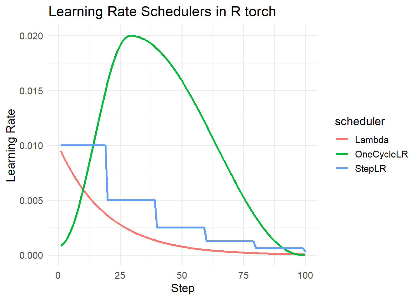
13.7 Concluding Remarks
There are a variety of means to potentially improve model performance or generalization. Here, we focused on a few common methods. However, this is a broad topic. Further, the field is continually advancing. We hope you find the methods that we discussed here useful. We will discuss other methods in the rest of this section specific to semantic segmentation tasks, such as data augmentations and adding specific modules to the archictecture. The deep learning process requires building an intuition for how to implement the training and validation processes, which is gained with experience.
13.8 Questions
- Explain how batch normalization is implemented after a convolutional layer.
- Explain the difference between the RMSprop and adam optimizers.
- Explain the difference between the adam and adamw optimizers.
- Explain the difference between the ReLU, leaky ReLU, and parameterized ReLU activation functions.
- Explain the concept of dying ReLU and why this is an issue.
- Explain the difference between the Dice and Tversky loss.
- If the goal is to train a multiclass classification model using imbalanced data, explain why macro-averaging to calculate the Dice loss is better than micro-averaging.
- Explain why CE loss is negatively impacted by class imbalance.
13.9 Exercises
Generate a function that will instantiate a scene labeling CNN architecture by subclassing nn_module(). The architecture should have a series of four 3x3 2D convolution + 2D batch normalization + activation function blocks. Following flattening, the vector should then pass through two fully connected + 1D batch normalization + activation function blocks. The last operation should be a fully connected layer with a number of neurons equal to the number of classes being differentiated. The user should be able to set the following components:
- Number of input layers or channels
- The number of classes being differentiated
- The number of output feature maps generated by each convolutional layer
- The kernel size for each convolution layer; a padding for each convolution layer should be applied so that the spatial dimensions are maintained regardless of the kernel size
- The number of neurons in the first two fully connected layers
- Whether or not to include batch normalization in the convolutional component of the architecture
- Whether or not to include batch normalization in the fully connected component of the architecture
- What activation function to use throughout the architecture (ReLU, leaky ReLU, or swish); if leaky ReLU is used, the user should be able to specify the negative slope term
- Whether or not to include dropout after the first two fully connected layers; if dropout is used, the user should be able to specify the probability
- Whether to return raw logits or re-scale the logits using a sigmoid or softmax function
Test your function using some random data of the correct shape.
Write documentation for your function that explains the required input spatial dimension sizes, general model architecture, and each user-defined parameter. A user should be able to use the documentation to implement your function.