1 Geospatial Raster Data Preprocessing (terra)
1.1 Topics Covered
- Reading raster geospatial data with terra.
- Raster preprocessing (crop, mask, merge, resample, and re-project)
- Raster math and logic
- Raster reclassification
- Raster summarization relative to points and polygons
- Rasterization of vector geospatial data (binary masks, Euclidean distance, kernel density)
1.2 Introduction
Since we primarily interact with our predictor variables for spatial predictive mapping and modeling tasks as raster grids, it is important to know how to work with and manipulate raster data in R. For this purpose, we will primarily make use of the terra package, which has superseded the raster package. In contrast to raster, terra does not require loading entire raster grids into memory. Instead, portions of data files can be loaded in as needed, which allows for processing large raster files. terra is also generally faster due to its reliance on C++.
terra introduces new classes for working with geospatial data in R:
-
spatRaster: raster data -
spatVector: geospatial vector data (points, lines, and polygons) -
spatExtent: extent or bounding box relative to a coordinate reference system (CRS).
Although the spatVector class allows for reading and working with vector data in R, we primarily use sf instead. An entire chapter, Chapter 24, is devoted to sf in the appendix section of the text.
The raster package had separate functions for reading in single band and multiband raster data. Single band data were read in with raster() while multiband data were read in with brick(). Multiple files could be referenced to a single multiband object using stack(). In contrast, in the terra package all raster data, no matter the number of bands, are read in using rast().
If you are interested in working with spatiotemporal arrays or data cubes in R, consider exploring the stars package. Since we will primarily work with single or multiband raster grids, we only discuss terra in this text.
Our primary goal in this section is to explore a wide variety of common raster preprocessing and analysis methods as implemented with terra. We will use tmap to visualize input data and results. tmap is discussed in Chapter 23.
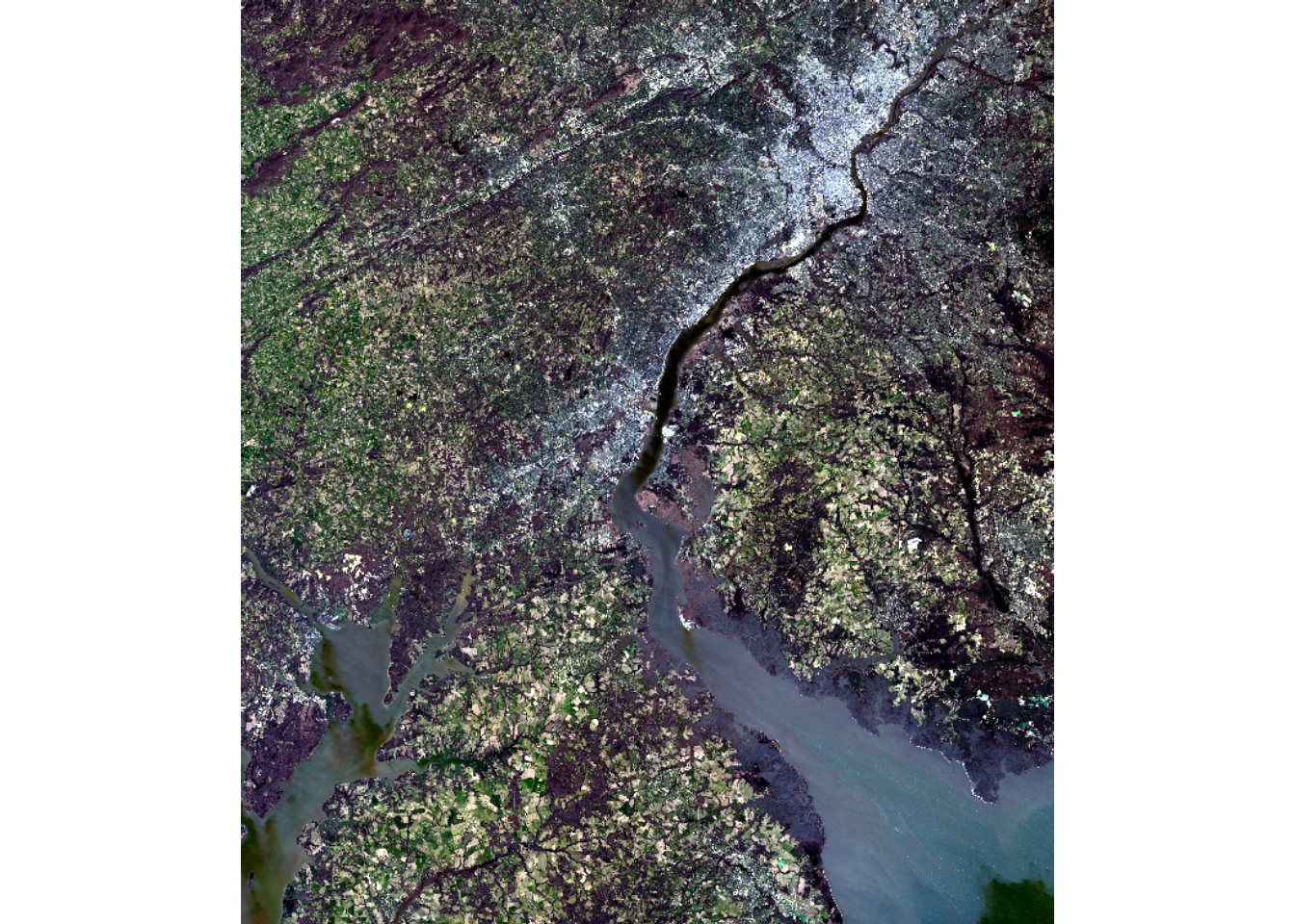
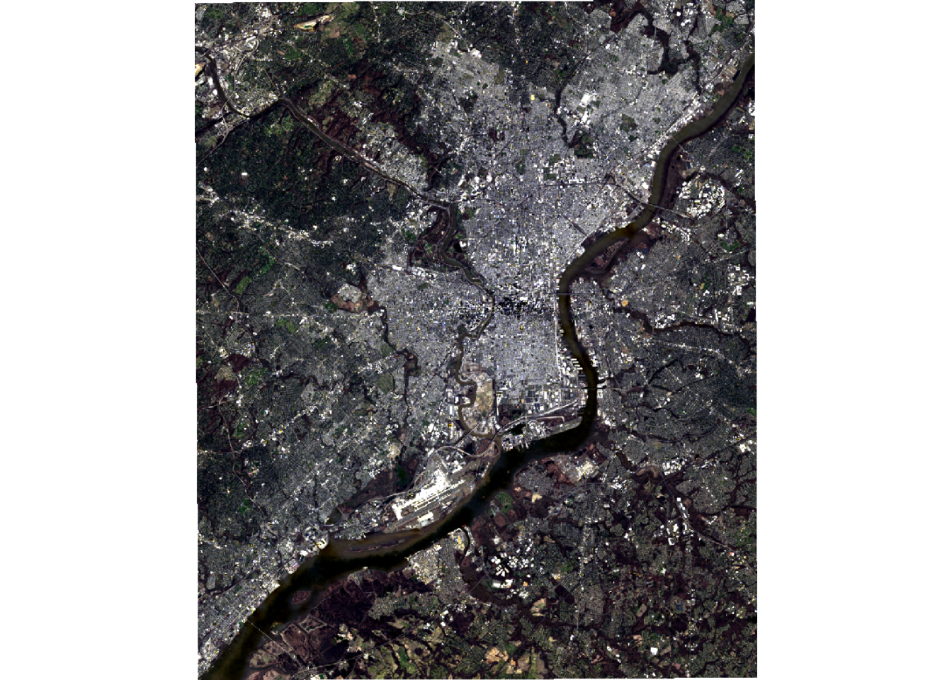
To support our demonstration, we read in several raster files. Using terra, raster data are read using the rast() function. We first load in a digital terrain model (DTM) from the United States Geological Survey (USGS) 3D Elevation Program (3DEP). In order to speed up our examples, we also degrade the raster by a factor of 5 and by calculating the mean of the 25 1x1 m cells within the new 5x5 m cells. This is accomplished using the aggregate() function from terra. We also read in multispectral data from the Landsat 8 Operational Land Imager (OLI) sensor. Using sf, we read in some vector extents, which will be used to crop out portions of the data, a county extent, sample point locations at which to extract raster cell values, and a hexagon tessellation, which will be used to demonstrate data summarization. The DTM data are visualized using tmap while the multiband data are visualized using the plotRGB() function from terra. In order to improve the visualization of the imagery, a linear stretch is applied (stretch="lin"). The imagery is displayed as a simulated true color image using the red, green, and blue bands. Lastly, the bands are renamed using the names() function and by providing a vector of band names in the correct order.
As is the standard in remote sensing and GIS, when we discuss the spatial resolution of a raster grid, instead of stating 5x5 m, we will use 5 m.
You should not need to update the folder paths below if you are accessing Quarto file from the downloaded directory. This is true for all chapters in the text. We assign the folder path to a variable near the start of each chapter.
fldPth <- "gslrData/chpt1/data/"

dtm <- rast(str_glue("{fldPth}dtm.tif")) |>
  aggregate(fact=5, fun=mean)

tm_shape(dtm)+
  tm_raster(style= "cont", palette=get_brewer_pal("-Greys", plot=FALSE))+
  tm_layout(legend.outside = TRUE)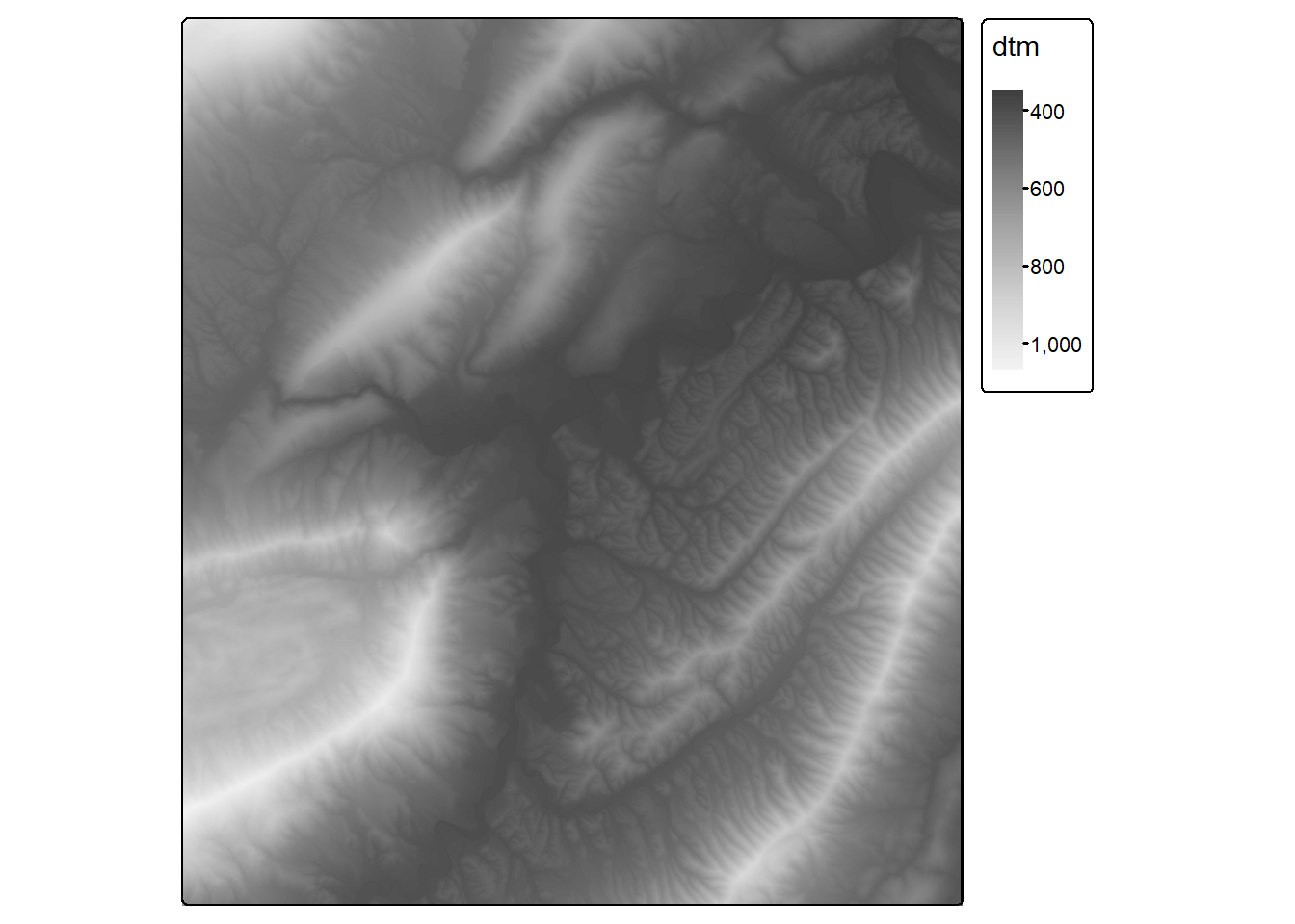
ext1 <- st_read(dsn=str_glue("{fldPth}chpt1.gpkg"),
                "extent1",
                quiet=TRUE)
ext2 <- st_read(dsn=str_glue("{fldPth}chpt1.gpkg"),
                "extent2",
                quiet=TRUE)
delawarCNT <- st_read(dsn=str_glue("{fldPth}chpt1.gpkg"),
                      "delawareCNTY",
                      quiet=TRUE)
sampPnts <- st_read(dsn=str_glue("{fldPth}chpt1.gpkg"),
                    "sampPnts",
                    quiet=TRUE)
tess <- st_read(dsn=str_glue("{fldPth}chpt1.gpkg"),
                "tesselation",
                quiet=TRUE)

names(lOff) <- c("Edge",
                 "Blue",
                 "Green",
                 "Red",
                 "NIR",
                 "SWIR1",
                 "SWIR2")
1.3 Raster Data Info
There are several functions that provide general information about raster data. The number of layers, channels, or bands can be obtained with nlyr(). The number of columns and rows of pixels or cells can be obtained with ncol() and nrow(), respectively. Lastly, coordinate reference information can be obtained with crs(). If proj=TRUE, the proj string is provided. If describe=TRUE, the CRS information is provided as a data frame. It is generally a good idea to explore your data before using them in an analysis.
nlyr(lOff)[1] 7ncol(lOff)[1] 3521nrow(lOff)[1] 4007crs(lOff)[1] "PROJCRS[\"AEA_WGS84\",\n BASEGEOGCRS[\"WGS 84\",\n DATUM[\"World Geodetic System 1984\",\n ELLIPSOID[\"WGS 84\",6378137,298.257223563,\n LENGTHUNIT[\"metre\",1]]],\n PRIMEM[\"Greenwich\",0,\n ANGLEUNIT[\"degree\",0.0174532925199433]],\n ID[\"EPSG\",4326]],\n CONVERSION[\"Albers Equal Area\",\n METHOD[\"Albers Equal Area\",\n ID[\"EPSG\",9822]],\n PARAMETER[\"Latitude of false origin\",23,\n ANGLEUNIT[\"degree\",0.0174532925199433],\n ID[\"EPSG\",8821]],\n PARAMETER[\"Longitude of false origin\",-96,\n ANGLEUNIT[\"degree\",0.0174532925199433],\n ID[\"EPSG\",8822]],\n PARAMETER[\"Latitude of 1st standard parallel\",29.5,\n ANGLEUNIT[\"degree\",0.0174532925199433],\n ID[\"EPSG\",8823]],\n PARAMETER[\"Latitude of 2nd standard parallel\",45.5,\n ANGLEUNIT[\"degree\",0.0174532925199433],\n ID[\"EPSG\",8824]],\n PARAMETER[\"Easting at false origin\",0,\n LENGTHUNIT[\"metre\",1],\n ID[\"EPSG\",8826]],\n PARAMETER[\"Northing at false origin\",0,\n LENGTHUNIT[\"metre\",1],\n ID[\"EPSG\",8827]]],\n CS[Cartesian,2],\n AXIS[\"easting\",east,\n ORDER[1],\n LENGTHUNIT[\"metre\",1,\n ID[\"EPSG\",9001]]],\n AXIS[\"northing\",north,\n ORDER[2],\n LENGTHUNIT[\"metre\",1,\n ID[\"EPSG\",9001]]]]"crs(lOff, proj = TRUE)[1] "+proj=aea +lat_0=23 +lon_0=-96 +lat_1=29.5 +lat_2=45.5 +x_0=0 +y_0=0 +datum=WGS84 +units=m +no_defs"crs(lOff, describe=TRUE) name authority code area extent
1 AEA_WGS84 <NA> <NA> <NA> NA, NA, NA, NAInformation about the raster layer can also be obtained by simply calling it, which is demonstrated below for the Landsat 8 OLI data (lOff). The number of rows, columns, and layers; spatial resolution; spatial extent; coordinate reference information; name of the source file; and the band names and range of values are also provided.
lOffclass : SpatRaster
dimensions : 4007, 3521, 7 (nrow, ncol, nlyr)
resolution : 30, 30 (x, y)
extent : 1673295, 1778925, 1975365, 2095575 (xmin, xmax, ymin, ymax)
coord. ref. : AEA_WGS84
source : ls8_3_11_2024_SR.tif
names : Edge, Blue, Green, Red, NIR, SWIR1, ...
min values : 0, 0, 0, 130, 5819, 6858, ...
max values : 63038, 62818, 65454, 65454, 64794, 65454, ... 1.4 General Data Processing
1.4.1 Band Subsets and Stacking
For a multiband raster grid, you can extract out a subset of the bands or layers using the band names and bracket notation. Data can be subsequently merged or stacked back to a single file using the c() function. terra is unforgiving in regards to differences in spatial extent, number of rows/columns of cells, and cell size. This is not an issue in our example since all the data being stacked were extracted from the same input grid.
imgStk <- c(visB, nirB, swirB)1.4.2 Crop, Mask, and Merge
The crop() function allows for extracting a rectangular extent from a larger raster file based on coordinates that define a bounding box. The coordinates can be created using the ext() function and should be relative to the projection of the data being cropped. The crop() function requires two arguments: the raster to be cropped and the extent. We plot the result to confirm that the extent has changed and print the raster information to confirm that there are now fewer columns and rows of cells in comparison to the original object. We repeat this process for a second extent in the second code block.
crop_ext1 <- ext(1710000, 1752000, 2030000, 20500000)
lOffCrop1 <- crop(lOff, crop_ext1)
plotRGB(lOffCrop1, r=4, g=3, b=2, stretch="lin")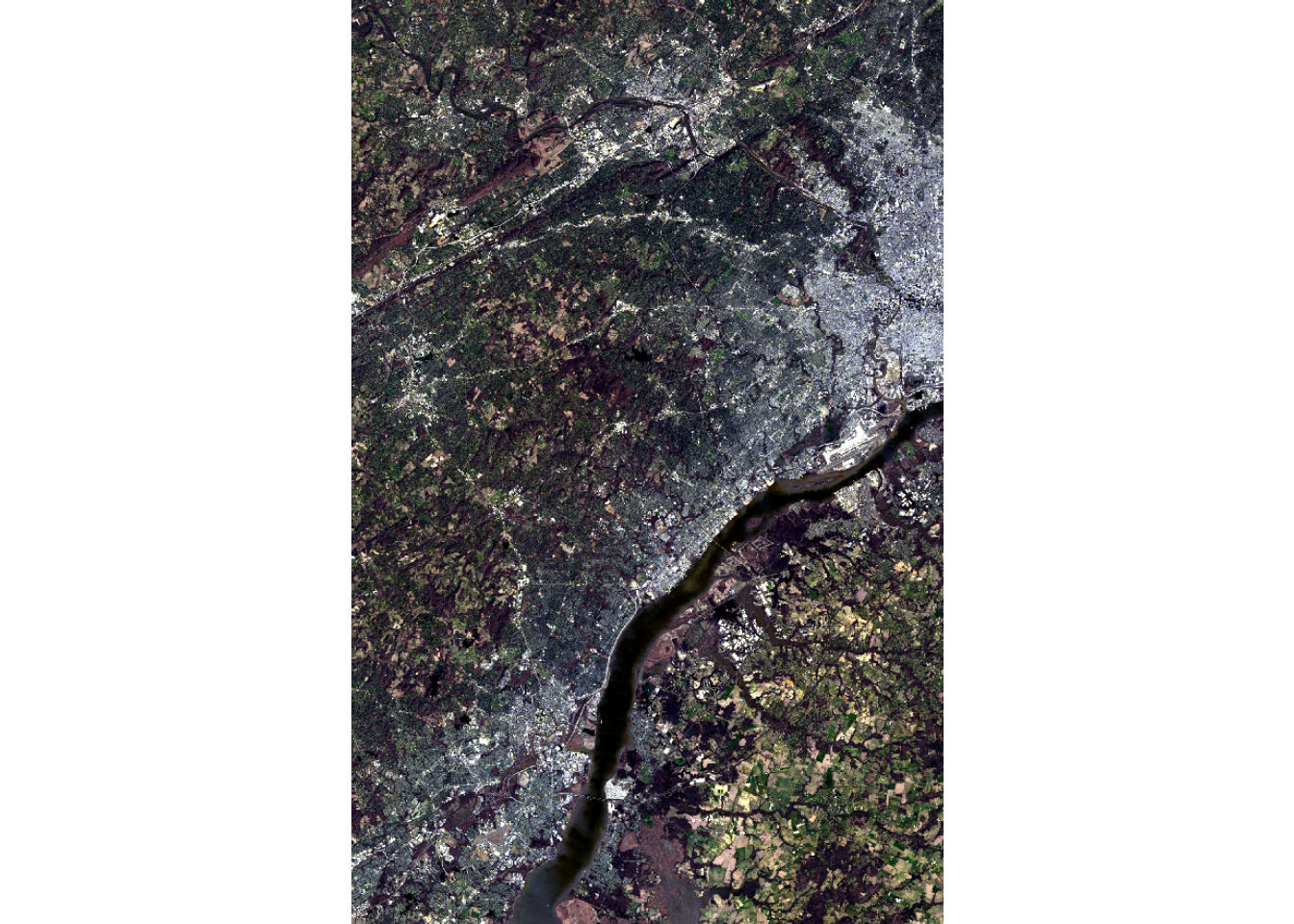
lOffCrop1class : SpatRaster
dimensions : 2186, 1400, 7 (nrow, ncol, nlyr)
resolution : 30, 30 (x, y)
extent : 1710015, 1752015, 2029995, 2095575 (xmin, xmax, ymin, ymax)
coord. ref. : AEA_WGS84
source(s) : memory
varname : ls8_3_11_2024_SR
names : Edge, Blue, Green, Red, NIR, SWIR1, ...
min values : 0, 0, 435, 1668, 6946, 6986, ...
max values : 59819, 61493, 65454, 65454, 64778, 65454, ... crop_ext2 <- ext(ext1)
lOffCrop2 <- crop(lOff, crop_ext2)
plotRGB(lOffCrop2, r=4, g=3, b=2, stretch="lin")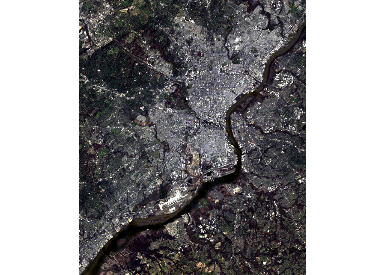
In contrast to crop(), mask() can be used to extract a non-rectangular extent. However, the resulting raster is still rectangular since each row and column of cells must have the same length or be a full array of values. mask() is simply converting cells outside of the mask to a NULL or NA assignment, which are displayed as transparent by default.
Below, we extract out two extents, one that is nearly rectangular and one that is circular. To demonstrate that NA cells exist for the circular extent, we assign a color to these cells when visualizing the data using the colNA argument.
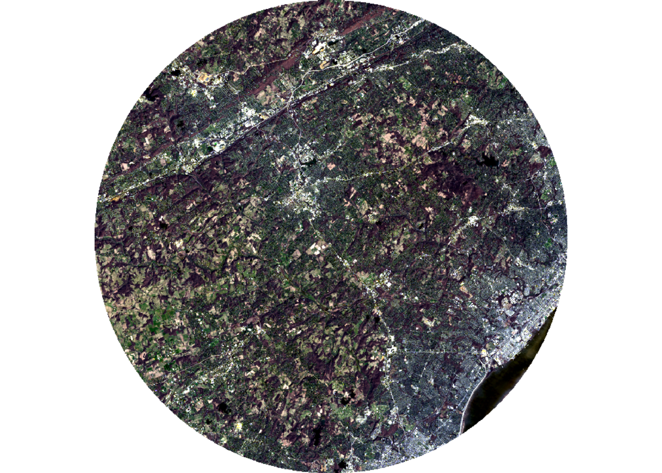
lOffCrop4 <- lOff |> crop(ext2) |> mask(ext2)
plotRGB(lOffCrop4, r=4, g=3, b=2, stretch="lin", colNA="salmon")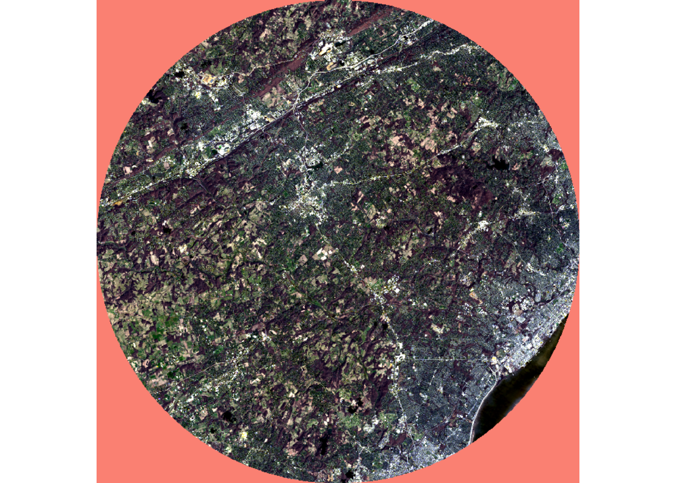
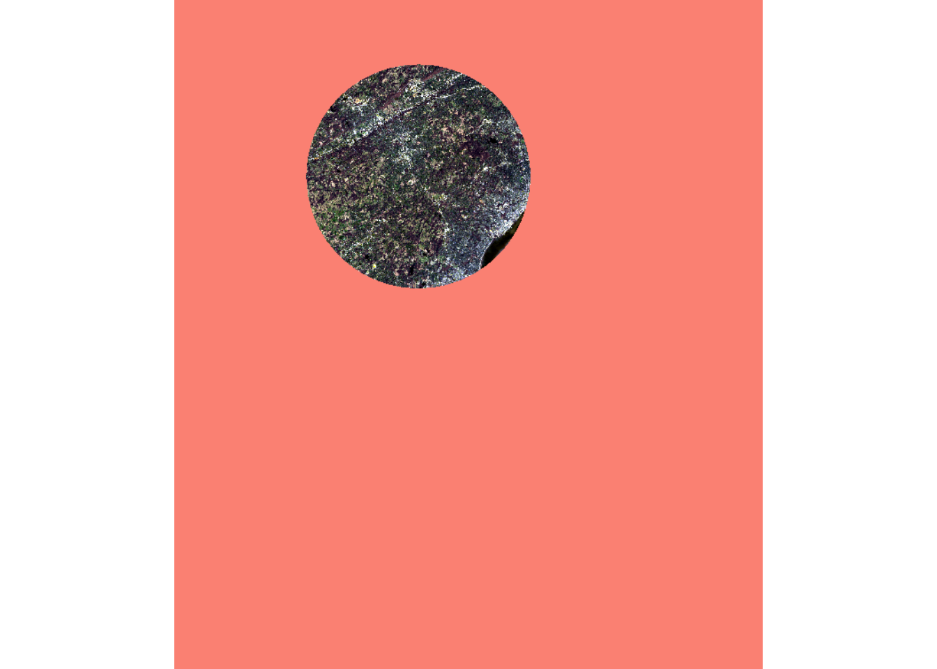
It is important to note that mask() does not remove rows and columns of cells; the function simply codes cells outside of the mask to NA. You may have noticed above that we used crop() followed by mask(). If we did not use crop(), as demonstrated in the next code block, all the original rows and columns of cells would have been maintained.
1.4.3 Resample
As noted above, terra is generally unforgiving when raster grids that are being used in the same operation have different numbers of rows and columns of cells, a different origin, different coordinate reference systems, and/or different cell sizes. In order to combat this issue, the resample() function can be used to align a grid to another grid. The first argument is the grid that is to be resampled while the second argument is the grid being used as a reference. A variety of resampling methods are available including nearest neighbor, bilinear interpolation, cubic convolution, cubic spline, and Lanczos windowed sinc. It is also possible to calculate a summary metric from the contributing cells, such as the mean.
When resampling categorical data, it is generally best to use nearest neighbor since any method that relies on averaging or weighted averaging is inappropriate for categorical data. For continuous data, such as image bands or DTMs, we commonly use either bilinear interpolation or cubic convolution.
1.4.4 Re-Project
If you need to change the coordinate reference system of a layer, or re-project the layer, you can use the project() function. This is appropriate when you know the current projection and the desired projection. This should not be used to set or define missing projection information. If the projection is missing, we first recommend troubleshooting the layer as there might be an issue with the file being referenced. If the project is known, it can be set using crs() then the layer can be subsequently re-projected using project() if desired.
1.4.5 Raster Math and Logic
Performing logical or mathematical operations on spatRaster objects is generally the same as performing such operations on a base R vector, matrix, or array.
In the first example, we are converting the DTM data from meters to feet units by simply multiplying each cell by the conversion factor.
elevFT <- dtm*3.28084When a logical operation is performed, the result will be a binary grid (0/1) where 0 indicates FALSE and 1 indicates TRUE. In our first example, we find all cells with an elevation greater than 700 m. In the second example, we find all cells in the result that were coded to 0, or were less than or equal to 700 m in elevation. This results in inverting the results: 0 returns 1 and 1 returns 0.
elev700 <- dtm > 700
tm_shape(elev700)+
  tm_raster(col.scale = tm_scale_categorical(labels = c("<= 700", "> 700"),
                                             values = c("gray", "darksalmon")))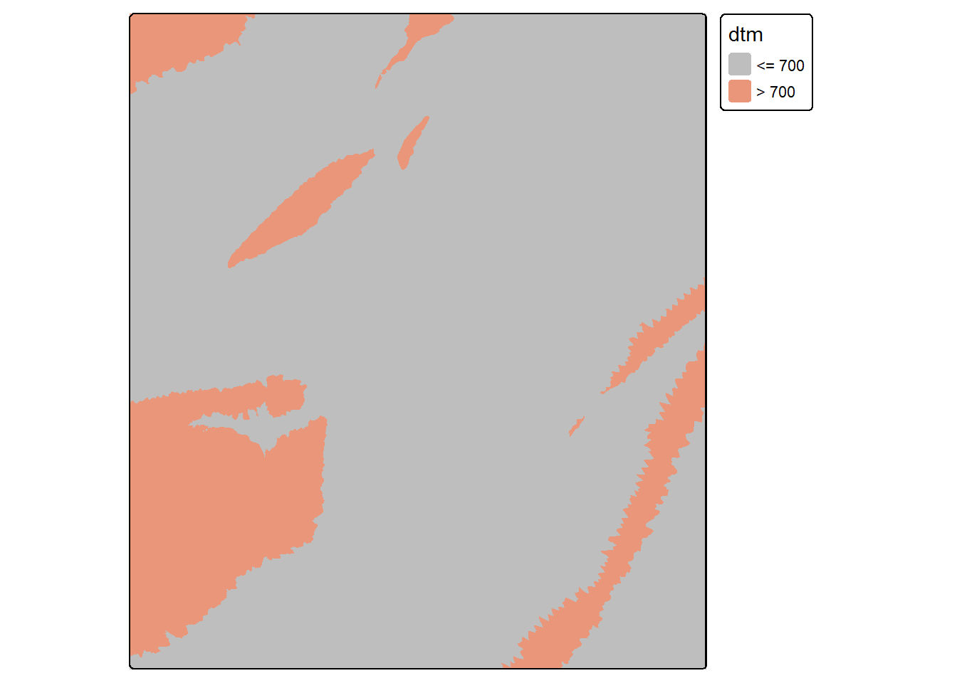
elev700b <- elev700 == 0
tm_shape(elev700b)+
  tm_raster(col.scale = tm_scale_categorical(labels = c("> 700", "<= 700"),
                                             values = c("gray", "darksalmon")))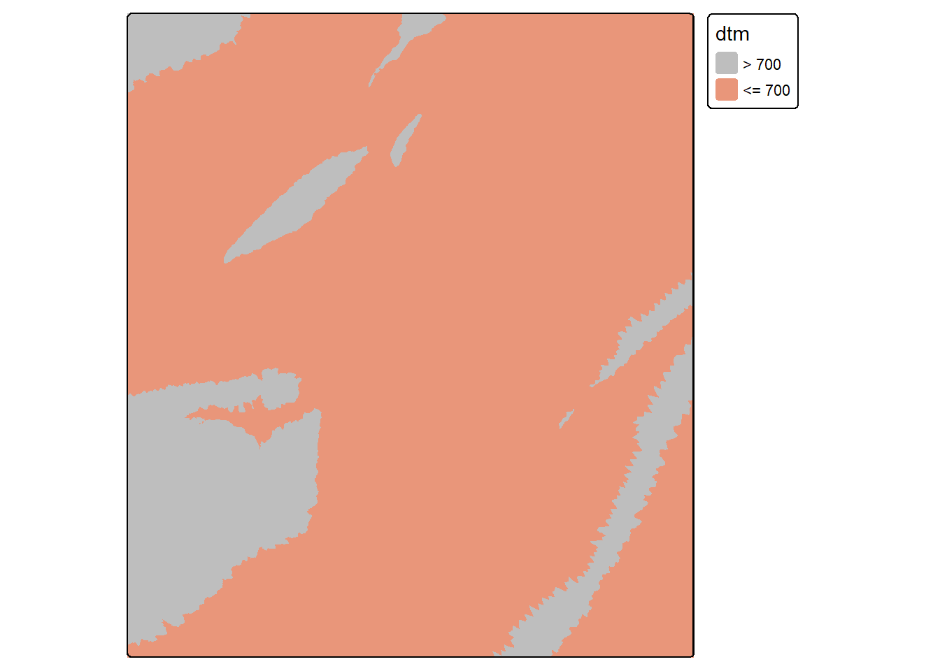
It is also possible to perform mathematical operations between two or more raster grids as long as they align, have the same cell size, and the same number of rows and columns of pixels. If they do not meet these criteria, then one grid should be resampled to match the other grid, as noted above. In our example below, we have multiplied the binary output by the original DTM to return a grid where all elevations less than or equal to 700 return 0 and all elevations greater than 700 return the original elevation.
rastMult <- elev700*dtm
tm_shape(rastMult)+
  tm_raster(style= "cont", palette=get_brewer_pal("-Greys", plot=FALSE))+
  tm_layout(legend.outside = TRUE)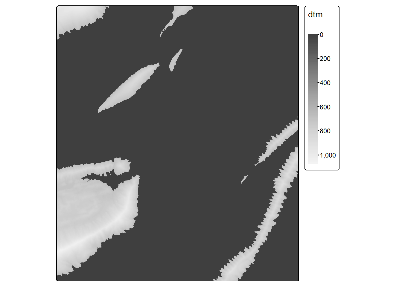
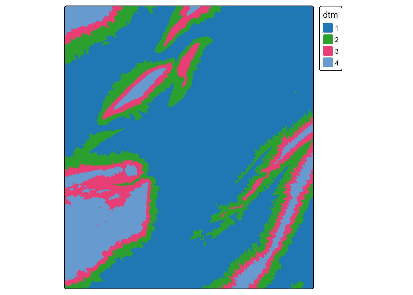
1.5 Reclassify
A categorical raster grid can be reclassified into a smaller number of categories. Alternatively, a continuous grid can be reclassified or binned into ranges. Using terra, this is accomplished with the classify() function; however, you must first define the desired reclassification scheme as a matrix. In our example, we have created a reclassification matrix with 3 columns. The first column is the starting value for the bin while the second column is the end value for the bin. The last column is the new cell value. So, in our example, values between 550 and 650 will be coded to 2. Inside of classify(), if right=TRUE, the interval is closed on the right and open on the left. This means that the high value in the range will code to that bin as opposed to the next bin.
If you are reclassifying categories or integers, you can use a matrix with only two columns where the first column references the original cell value and the second column references the new cell value.
1.6 Data Summarization
There are many situations where you may want to extract raster cell values at point locations. For example, this could be used to create tabulated data to perform a correlation analysis or data visualization. This process can also be useful for creating training data for supervised learning projects, which is the focus of this text.
Our first example below demonstrates how to extract raster values at point locations using the extract() function from terra. In our example, we have extracted the raster channel cell values at point locations then merged the results back to the original point layer using dplyr. The geometry information is removed prior to adding the results back to the original point layer using geom=NULL within as.data.frame(). The new columns in the table use the band names from the image data.
pnts <- terra::extract(lOff, sampPnts) |>
  as.data.frame(geom=NULL)
sampPnts1 <- bind_cols(sampPnts, pnts)

head(sampPnts1)
Simple feature collection with 6 features and 9 fields
Geometry type: POINT
Dimension: XY
Bounding box: xmin: 1686721 ymin: 2077187 xmax: 1748325 ymax: 2083037
Projected CRS: AEA_WGS84
Id ID Edge Blue Green Red NIR SWIR1 SWIR2 Shape
1 0 1 8356 8684 10020 10077 20599 14940 11568 POINT (1686721 2077187)
2 0 2 7966 8076 8475 8297 7916 7788 7629 POINT (1701710 2077370)
3 0 3 9117 9361 10012 10317 15480 15965 13325 POINT (1714141 2079015)
4 0 4 8415 8534 8984 9047 13219 12344 10663 POINT (1730959 2078832)
5 0 5 8173 8221 8463 8652 10881 12026 10538 POINT (1739551 2083037)
6 0 6 10393 10919 11223 11829 13969 13951 12781 POINT (1748325 2082123)If is also possible to perform a summarization relative to polygon extents. In such cases, you will need to specify what statistic to calculate from the cells occurring within the extent of each polygon. In our example, we are calculating the median (fun=median). Once the data are extracted, new measures can be generated in the table using basic table manipulation. Below, we calculate the normalized difference vegetation index (NDVI) using the near infrared (NIR) and red bands and mutate() from dplyr.
To visualize the results, we display the median NDVI value for each hexagon in the tessellation.
tessSummary <- terra::extract(lOff, tess, fun=median) |>
  as.data.frame(geom=NULL)

tessSummary <- tessSummary |>
  mutate(ndvi = ((NIR-Red)/(NIR+Red+0.001)))

tess <- bind_cols(tess, tessSummary)

tm_shape(tess)+
  tm_polygons(fill="ndvi",
              fill.scale = tm_scale_continuous(values="brewer.greens"),
              fill.legend = tm_legend(title="Median NDVI"))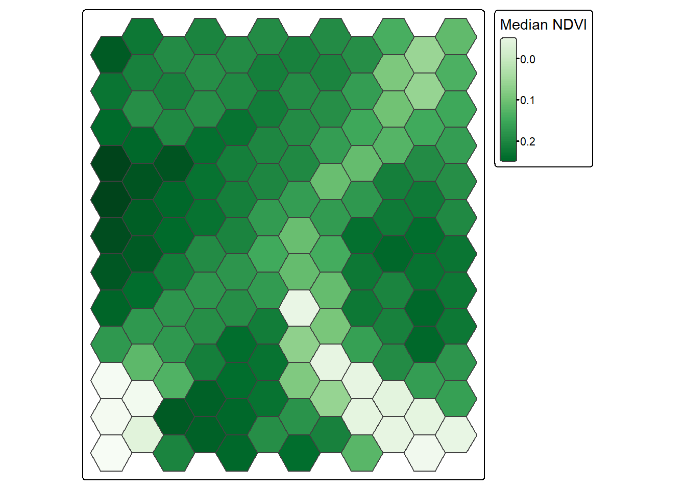
If you would like to generalize the extracted information for each point sample, you could use a buffered version of the points and calculate a statistic from all the cells that fall within the buffer, which is demonstrated below. Alternatively, you could perform a smoothing or generalization of the raster data prior to summarizing them.
pnts <- terra::extract(lOff, st_buffer(sampPnts, 200), fun=mean) |>
  as.data.frame(geom=NULL)
sampPnts2 <- bind_cols(sampPnts, pnts)

head(sampPnts2)
Simple feature collection with 6 features and 9 fields
Geometry type: POINT
Dimension: XY
Bounding box: xmin: 1686721 ymin: 2077187 xmax: 1748325 ymax: 2083037
Projected CRS: AEA_WGS84
Id ID Edge Blue Green Red NIR SWIR1 SWIR2
1 0 1 8347.460 8661.935 9884.683 9825.273 20057.02 14739.43 11535.76
2 0 2 8308.529 8557.514 9244.312 9497.732 11898.66 12162.55 10437.28
3 0 3 8718.957 8910.304 9521.283 10009.812 14725.14 15559.21 12869.01
4 0 4 8354.420 8535.818 9144.930 9156.056 14890.20 12931.71 10900.47
5 0 5 8323.145 8444.101 8879.841 9140.457 13140.59 13664.43 11493.73
6 0 6 9954.129 10343.564 10989.979 11397.186 13723.26 13809.34 12630.51
Shape
1 POINT (1686721 2077187)
2 POINT (1701710 2077370)
3 POINT (1714141 2079015)
4 POINT (1730959 2078832)
5 POINT (1739551 2083037)
6 POINT (1748325 2082123)1.7 Ancillary Data
You may want to incorporate information derived from vector data into your model as predictor variables or as a processing mask. For example, if your results only pertain to land, you may want to mask out all water areas in the final result. There are several means to represent vector data in a raster format. For categories, unique numeric codes can be used to differentiate categories on a cell-by-cell basis. You may also be interested in representing the distance from features or the density of features. These methods are demonstrated below; however, we first need to read in some example data. Here, we make use of data for Morgantown, West Virginia, USA provided by the West Virginia GIS Technical Center. These layers include public land extents, wards or subdivisions of the city, buildings as point locations, and roads as line features. Before working with these data, we visualize them using tmap.
folderPath <- "gslrData/chpt1/data/morgantown/"

pLands <- st_read(str_glue("{folderPath}publicLands.shp"),
                  quiet=TRUE)
wards <- st_read(str_glue("{folderPath}wards.shp"),
                 quiet=TRUE)
strPnts <- st_read(str_glue("{folderPath}structures.shp"),
                   quiet=TRUE)
rds <- st_read(str_glue("{folderPath}roads.shp"),
               quiet=TRUE)
moTownMap1 <- tm_shape(wards)+
tm_polygons(fill="tan")+
tm_shape(pLands)+
tm_polygons(fill="darkolivegreen")
moTownMap2 <- tm_shape(wards)+
tm_polygons(fill="tan")+
tm_shape(strPnts)+
tm_dots(fill="red",
size=.2)
moTownMap3 <- tm_shape(wards)+
tm_polygons(fill="tan")+
tm_shape(rds)+
tm_lines(col="black")
tmap_arrange(moTownMap1, moTownMap2, moTownMap3)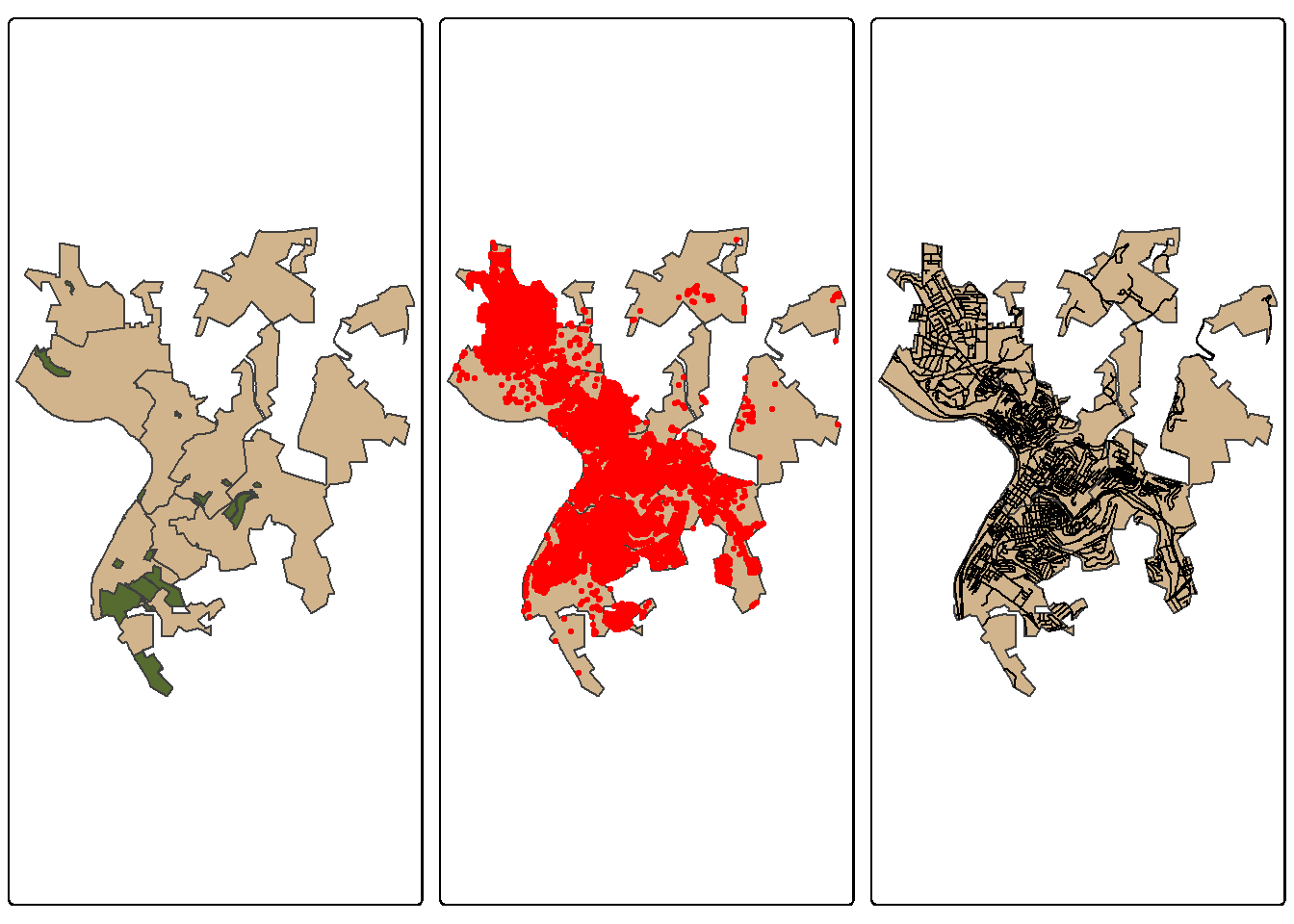
1.7.1 Rasterization
First, we convert the public land data into a binary raster mask. We first need to generate a template raster. This is accomplished using rast(). We specifically create a raster that fills the spatial extent of the wards layer, has a resolution of 10 m, and uses the same CRS as the wards layer.
We would first like all of the cells within the extent of the wards to be coded to 0. To accomplish this, we first create a new column in the attribute table that holds the value 0 for each record. The rasterize() function is used to convert these data to a raster using the column with the zero code and the template raster that was already generated. All cells outside of the wards extent but within the associated layers bounding box are coded to NA.
We next repeat this process for the public lands layer but using a cell value of 1. By adding the results, we obtain a raster grid where areas within public lands and within the ward extents are coded to 1, cells within the wards extents but not in the public lands are coded to 0, and cells within the bounding box extent but not within the wards are coded to NA.
rTemplate <- rast(ext(wards),
                  res = 10,
                  crs = crs(wards))

wards$code <- 0
wardsR <- rasterize(wards,
                    rTemplate,
                    field = "code",
                    background = NA,
                    touches = TRUE)

pLands$code <- 1
pLandsR <- rasterize(pLands,
                     rTemplate,
                     field = "code",
                     background = 0,
                     touches = TRUE)+wardsR

tm_shape(pLandsR)+
  tm_raster(col.scale = tm_scale_categorical(labels = c("Private", "Public"),
                                             values = c("darkgrey", "darkolivegreen")),
            col.legend = tm_legend(title="Private vs. Public"))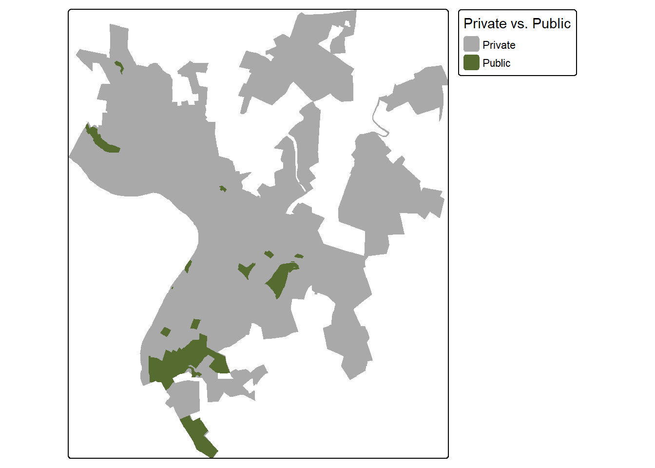
1.7.2 Distance Grids
Euclidean, or straight-line, distance from the nearest vector feature can be generated using the distance() function from terra. This function also requires a template raster. So that our result aligns with the public land mask created above, we use the same template raster. The resulting distances are in the map units, in this case meters.
In order to mask the result to the ward extents, we add the distance and ward raster grids. Since all cells in the wards are coded to 0, adding this does not change the distance measurement. However, this converts all of the cells outside of the ward extents to NA since adding NA to any other value always returns NA.
rdDist <- distance(wardsR, rds)+wardsR

tm_shape(rdDist)+
  tm_raster(col.scale = tm_scale_continuous(values="brewer.reds"),
            col.legend = tm_legend(title="Distance (m)"))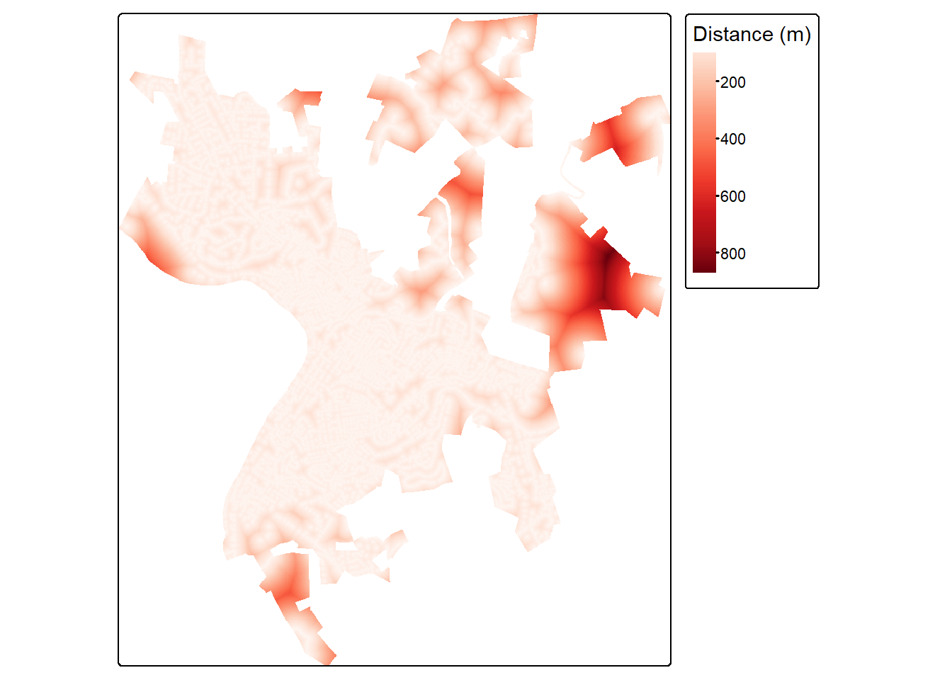
1.7.3 Density Grids
For point data, you may be interested in calculating the density of features as opposed to the distance from the nearest features. This can be accomplished using the sf.kde() function from the spatialEco package. This is demonstrated below for the building point features. The bandwidth (bw) determines the size of the window used for the kernel density calculations. Larger values result in a more generalized pattern while smaller values result in a more local pattern. We are also using the wards extent to mask the results just as we did for the distance grid above.
strDensity <- sf.kde(strPnts,
                     bw=200,
                     ref=wardsR,
                     res=10)+wardsR
[1] 200tm_shape(strDensity)+
tm_raster(col.scale = tm_scale_continuous(values="brewer.purples"),
col.legend = tm_legend(title="Structure Density"))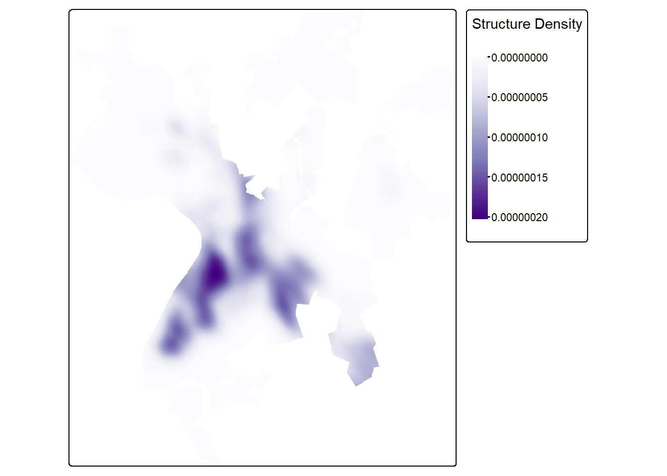
1.8 Concluding Remarks
We use raster data throughout the text, so you will see the general methods discussed in this chapter often. The terra package has a variety of functions available, and we only discussed a small percentage of them here. Please consult its documentation for further exploration. In the next chapter, we specifically focus on preprocessing multispectral data and DTMs to generate data augmentations or additional predictor variables.
1.9 Questions
- Explain the difference between
crop()andmask(). - Explain the difference between raster aggregation and raster resampling.
- Why is bilinear interpolation and cubic convolution not appropriate resampling methods for categorical raster data?
- Using terra, explain a method that can be used to force two raster grids to align and have the same number of rows and columns of cells.
- Explain the purpose of the
rightparameter for theclassify()function from terra. - Explain the purpose/use of the
crosstab()function from terra. - Explain the purpose/use of the
clamp()function from terra. - Explain the purpose/use of the
disagg()function from terra.
1.10 Exercises
Goal
You have been provided with a set of files that need to be processed to generate a conservative suitability model and a liberal suitability model. The provided files are in the exercise folder for the chapter and include:
- chpt1.gpkg/extent: study area extent as a polygon feature
- chpt1.gpkg/watersheds: watershed boundaries within study area extent
- slp.tif: raster grid of topographic slope in degrees
- dtm.tif: raster grid of elevation in meters
- lc2.tif: land cover classes from the National Land Cover Database (NLCD) 2024
- strmD.tif: distance from streams in meters
All data are projected to NAD83 UTM Zone 17N. All raster grids have a resolution of 30 m.
Preprocessing
Perform the following pre-processing tasks.
- Read in all the data layers
- Crop and mask the the elevation data relative to the extent polygon
- Align the topographic slope, land cover, and stream distance grids with the elevation grid. Use nearest neighbor for the land cover and cubic convolution for the slope and stream distance grids
- Use tmap to create map layouts of all four raster grids. Merge them into a single layout using
tmap_arrange().
Conservative Model
- Generate the following binary grids:
- Mixed or deciduous land cover = 1; all other cover types = 0. (The NLCD legend can be found here)
- Elevations > 900 m = 1; elevations <= 900 m = 0
- Topographic slope < 30 degrees = 1; topographic slope >= 30 degrees = 0
- Distance from stream < 150 m = 1; distance from stream >= 150 m = 0
- Find all cells that meet all 4 criteria in the study area extent (suitable = 1; not suitable = 0)
- Create a map layout of your result using tmap
- For each watershed in the extent, calculate the total area suitable in hectares and the percent of suitable area
- Create a map layout of your result
Liberal Model
- Create grids linearly scaled between 0 and 1 such that the most suitable value is coded to 1 and the least suitable value is coded to 0.
- Higher elevations most suitable
- Lower topographic slopes most suitable
- Closer to stream most suitable
- Re-code the the land cover data as follows:
- Deciduous forest = 0.5
- Evergreen forest = 1.0
- Mixed forest = 0.75
- Woody wetland = 0.25
- All other types = 0
- Multiply all four results to obtain a combined suitability
- Re-scale the output from 0 to 1.
- Make a map layout of the results using tmap
- Summarize the mean suitability for each watershed
- Make a map layout of the watershed-scale mean suitability using tmap