4 Lidar Processing (lidR)
4.1 Topics Covered
- Working with light detection and ranging (lidar) data using lidR
- Point cloud reading, filtering, and preprocessing
- Point cloud rasterization
- Point cloud summarization at the cloud-, field plot-, and pixel-levels
- Processing using LAS Catalogs
4.2 Introduction
Light detection and ranging (lidar) data can offer unique information to compliment other remotely sensed and geospatial input data for spatial predictive mapping and modeling. For example, aerial systems that are capable of capturing multiple returns from a single laser pulse offer a means to at least partially characterize the vertical structure of vegetation, information that is not readily available from spectral data. Lidar is also a common data source to generate digital terrain models (DTMs) and subsequent land surface parameters (LSPs), as were discussed in Chapter 2, often with a high degree of local detail.
This chapter explores the processing of lidar point clouds using the lidR package. The package includes excellent and detailed documentation. In this single chapter, we are unable to cover the package in the same level of detail as that offered by this documentation. If you are interested in learning more about lidar processing using lidR, we highly recommend checking out this documentation.
Since our primary focus here is generating predictor variables for us in spatial predictive mapping and modeling, we focus on aspects of lidar processing most applicable to these tasks. Some components of lidR are not discussed or only discussed briefly, including ground return classification, tree identification, and tree crown segmentation. Our primary focus is reading and preparing data; generating raster derivatives; and summarizing the point cloud at the cloud-, plot-, and pixel-levels.
Other than lidR, we read in sf for handling vector geospatial data, terra for handling raster geospatial data, the tidyverse for general data wrangling, tmap/tmaptools for mapping and spatial data visualization, and gt for generating tables.
4.3 Reading, Preparation, and Filtering
For our example, we will process lidar data provided by the United States Geological Survey (USGS) 3D Elevation Program (3DEP) for the area around the town of Monticello in southern Utah, USA. These data were downloaded using OpenTopography. If you use digital elevation data, we highly recommend checking out OpenTopography. It provides access to a wide variety of lidar data and derivatives along with tools for processing point clouds and DTMs.
Only three data layers are required:
- monticelloExtent.shp: study area extent polygon
- fieldPlots.shp: point features representing 15 hypothetical field plot locations
- points.laz: aerial point cloud data
We use tmap to display the vector layers over an ESRI imagery base map in the code block below.
monticello <- st_read("gslrData/chpt4/data/monticelloExtent.shp", quiet = TRUE)

fPlts <- st_read("gslrData/chpt4/data/fieldPlots.shp", quiet=TRUE)

tm_shape(monticello)+
  tm_borders()+
  tm_basemap("Esri.WorldImagery")+
  tm_borders(col="red", lwd=2)+
  tm_shape(fPlts)+
  tm_bubbles(fill="yellow", size=.5)+
  tm_scalebar(position = tm_pos_out("center",  "bottom"),
               text.size = 1) +
  tm_compass (type = "arrow",
              size = 2,
position = tm_pos_out("right", "bottom")) 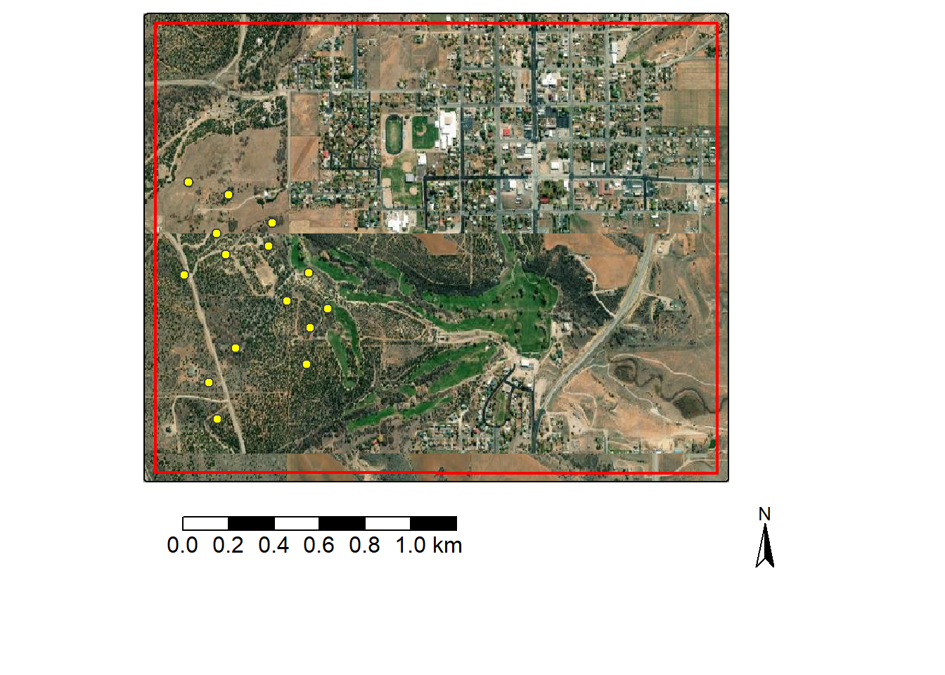
In order to select out a subset of the point cloud data, we extract the bounding box coordinates for the study area extent polygon using st_bbox() from sf. All data, including the lidar point cloud, are referenced to the WGS84 UTM Zone 12N coordinate reference system, so the extent represents easting and northing measurements.
     xmin      ymin      xmax      ymax
 644077.0 4191186.1  646578.8 4193195.4
It is common to want to use only a subset of an available point cloud. This could be a spatial subset and/or returns that meet certain criteria. For example, you may only be interested in first returns or ground returns. Using lidR, there are two general means to filter or subset points. One option is to read in the entire dataset then use filtering or clipping functions to subset the desired points. Table 4.1.provides a list of lidR filtering functions with associated explanations while Table 4.2 describes functions for extracting a spatial subset.
These methods work; however, it is generally more memory efficient and faster to perform the filtering when the data are read in so that data that will never be used are not stored in memory. Another means to reduce memory consumption is to only read in attributes that are required. Attributes can be selected using the abbreviations described in Table 4.3.
| Filter | Use |
|---|---|
filter_poi() |
Use query |
filter_first() |
First returns |
filter_firstlast() |
First and last returns |
filter_firstofmany() |
First of many returns |
filter_ground() |
Ground classified |
filter_last() |
Last returns |
filter_nth() |
Based on return number |
filter_single() |
Single returns |
filter_duplicates() |
Find duplicates |
| Function | Description |
|---|---|
clip_roi() |
Clip based on vector geometry (e.g., sf object) |
clip_rectangle() |
Clip based on rectangular extent defined by x-left, y-bottm, x-right, and y-top coordinates |
clip_circle() |
Clip based on circular extent defined by x- and y-center coordinates and a radius |
clip_transect() |
Clip along a transect between two points and using a given width |
| Attribute | Description |
|---|---|
| x | X coordinate |
| y | Y coordinate |
| z | Z coordinate (elevation) |
| i | Return intendity |
| t | GPS time |
| a | Scan angle |
| n | Number of returns associated with pulse |
| r | Return number |
| c | Classification |
| s | Synthetic data flag |
| k | Keypoint flag |
| w | Withheld flag |
| o | Overlap flag |
| p | Point source ID |
| e | Edge of flight line flag |
| d | Direction of scan flag |
The code below provides an example of using the select and filter arguments within the readLAS() function to subset the data when it is read in. This technique makes use of flags to select a subset of the points. In the example, we are reading in two copies of the data: one for all of the returns and one for just the ground returns. For each set, we only read in the x, y, and z coordinates; return intensity; classification; and return number. For all returns, we do not read in any withheld data points, which generally represent outliers, and only points that fall within the study area bounding box extent, which is defined using the bounding box coordinates obtained above. For the ground points, the same attributes are read in, and we only need to add one more flag to obtain only the ground points: -keep_class 2. This works because 2 is the classification assigned to ground returns.
The example lidar data use the .laz format. This is a compressed version of the .las file. lidR is capable of reading in both .laz and .las files.
lidR provides more specific read functions for different types of point cloud data. readALSLAS() is designed for reading in aerial lidar data, readTLSLAS() is designed for reading in data collected with a terrestrial laser scanner (TLS), and readUAVLAS() is designed for data collected from an unpiloted aerial vehicle platform. The main difference is that they can use different presets for certain lidR functions and processes. We use the more generic readLAS() function here.
More information about the available filtering flags can be obtained with readLAS(filter = "-help").
The point cloud data are stored in an S4 LAS object, which has two primary components: @head stores information and metadata about the file while @data stores the point data and associated attributes. Printing the names of the columns in @data, we can see that only the selected fields have been read in. We also print the first few rows of @data to see the structure of the table. Further, the number of returns in each dataset is equivalent to the number of rows in @data. The all returns set contains nearly ~18 million points while the ground subset contains ~10.5 million points.
names(lasAll@data)[1] "X" "Y" "Z" "Intensity"
[5] "ReturnNumber" "Classification"| X | Y | Z | Intensity | ReturnNumber | Classification |
|---|---|---|---|---|---|
| 646430.9 | 4193103 | 2137.37 | 24939 | 1 | 2 |
| 646430.8 | 4193102 | 2137.31 | 20864 | 1 | 2 |
| 646430.8 | 4193101 | 2137.40 | 18582 | 1 | 2 |
| 646430.8 | 4193099 | 2137.33 | 27384 | 1 | 2 |
| 646430.7 | 4193098 | 2137.34 | 26895 | 1 | 2 |
| 646430.7 | 4193097 | 2137.66 | 24287 | 1 | 2 |
data.frame(Set = c("All", "Ground Returns"),
           Counts = c(nrow(lasAll@data),
                      nrow(lasGrd@data))) |>
  gt() |>
  fmt_number(
    columns = Counts,
    decimals = 0,
use_seps = TRUE)| Set | Counts |
|---|---|
| All | 17,903,378 |
| Ground Returns | 10,579,821 |
The summary() function returns additional information about the point cloud including the size of the data in memory, its spatial extent and coordinate reference system, the area covered, the number of returns, and the average point and pulse density.
summary(lasAll)The developers of lidR highly recommend that the data be checked prior to use. This is accomplished with the las_check() function. Although some checks are performed when the data are read, las_check() conducts a more thorough check. One issue noted is duplicate measurements; as a result, we remove duplicates using filter_duplicates() before proceeding.
las_check(lasAll)
 Checking the data
  - Checking coordinates... ✓
  - Checking coordinates type... ✓
  - Checking coordinates range... ✓
  - Checking coordinates quantization... ✓
  - Checking attributes type... ✓
  - Checking ReturnNumber validity... ✓
  - Checking NumberOfReturns validity... ✓
  - Checking ReturnNumber vs. NumberOfReturns... ✓
  - Checking RGB validity... ✓
  - Checking absence of NAs... ✓
  - Checking duplicated points...
    ⚠ 4716 points are duplicated and share XYZ coordinates with other points
  - Checking degenerated ground points...
    ⚠ There were 459 degenerated ground points. Some X Y Z coordinates were repeated
    ⚠ There were 232 degenerated ground points. Some X Y coordinates were repeated but with different Z coordinates
  - Checking attribute population... ✓
  - Checking gpstime incoherances skipped
  - Checking flag attributes... ✓
  - Checking user data attribute... skipped
 Checking the header
  - Checking header completeness... ✓
  - Checking scale factor validity... ✓
  - Checking point data format ID validity... ✓
  - Checking extra bytes attributes validity... ✓
  - Checking the bounding box validity... ✓
  - Checking coordinate reference system... ✓
 Checking header vs data adequacy
  - Checking attributes vs. point format... ✓
  - Checking header bbox vs. actual content... ✓
  - Checking header number of points vs. actual content... ✓
  - Checking header return number vs. actual content... ✓
 Checking coordinate reference system...
  - Checking if the CRS was understood by R... ✓
 Checking preprocessing already done
  - Checking ground classification... yes
  - Checking normalization... no
  - Checking negative outliers... ✓
  - Checking flightline classification... skipped
 Checking compression
  - Checking attribute compression... no
lasAll <- lasAll |> filter_duplicates()
lasGrd <- lasGrd |> filter_duplicates()Point cloud data can be visualized using a dynamic, interactive 3D viewer using the plot() function. The code below was not executed when this chapter was rendered since the 3D view cannot be embedded in the web document. However, you can run it in RStudio to see the result. We specifically are displaying the return intensity using a grayscale color ramp.
gr_pal <- function(n) gray.colors(n, start = 0, end = 1)

plot(lasAll,
     color = "Intensity",
     pal= gr_pal,
     breaks = "quantile",
     bg = "white")
Next, we explore the distribution of the z or elevation values in the all returns set using a histogram. This suggests that there are still some high outlier points; as a result, we further filter the data using filter_poi() to remove any returns with a z greater than 2,300 meters. At this point, the data have been cleaned and are ready for use.
lasAll@data |>
  ggplot(aes(x=Z))+
  geom_histogram()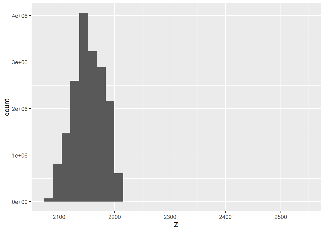
lasAll <- lasAll |> filter_poi(Z < 2300)4.4 Rasterization
Raster grids can be generated from point cloud data. Examples include the following:
- Digital terrain model (DTM): raster of bare earth surface elevations
- Digital surface model (DSM): raster that includes above ground features, such as trees and buildings, in the elevation surface
- Normalized digital surface model (nDSM): DSM - DTM; height of features above the ground surface
In order for a DTM to be generated from a point cloud, a ground classification must be performed. lidR provides implementations of several ground classification algorithms. You can read more about them in Chapter 4 of the lidR documentation. The data set we are using has already had ground classification performed, so this step is note necessary in our case. Ground classification is commonly performed by the vendor using a combination of algorithms and manual editing. As a result, it is not expected that using only an algorithm, such as those made available in lidR, will be able to produce a ground classification of comparable quality to those generated by data originators. However, they can be useful if a ground classification has not been performed and there is not adequate time to incorporate manual methods.
When only trees or vegetation are included as above ground features in the point cloud, a generated nDSM is commonly termed a canopy height model (CHM) since all above ground heights can be attributed to vegetation. However, this requires the classification of vegetation returns, which is a difficult task in many landscapes. Chapter 8 in the lidR documentation discusses tree identification and canopy segmentation algorithms implemented in lidR. Since we are not attempting to differentiate vegetation from other above ground features, such as buildings, in our example, we are creating an nDSM as opposed to CHM.
A DTM is generated using only the ground returns. The rasterize_terrain() algorithm requires input ground data or a point cloud with a ground classification performed, an output cells size, and an interpolation algorithm. lidR implements triangulated irregular network (TIN), k-nearest neighbor inverse distance weighting, and kriging interpolation methods. We generally recommend experimenting with different algorithms to determine which works best for your use case or landscape. Here, we use the k-nearest neighbor inverse distance weighting method implemented with the knnidw() function. When using this algorithm, the user can specify the number of neighbors to use (k), the power used to apply inverse distance weighting (p), and the maximum search radius (rmax).
In our example, we use a cell size of 5 m (i.e., 5-by-5 m cells), up to 10 neighbors, a power of 2, and the default search radius (50 meters). The result is a spatRaster() object. We plot the DTM with tmap. To further explore the data, we use terra to create a hillshade then display the elevation data over the hillshade.
dtm <- rasterize_terrain(lasGrd,
                         res=5,
                         algorithm=knnidw(k = 10L,
p = 2))tm_shape(dtm)+
tm_raster(col.scale = tm_scale_continuous(values="kovesi.linear_gow_65_90_c35"),
col.legend = tm_legend(orientation= "landscape",
title="Elevation"))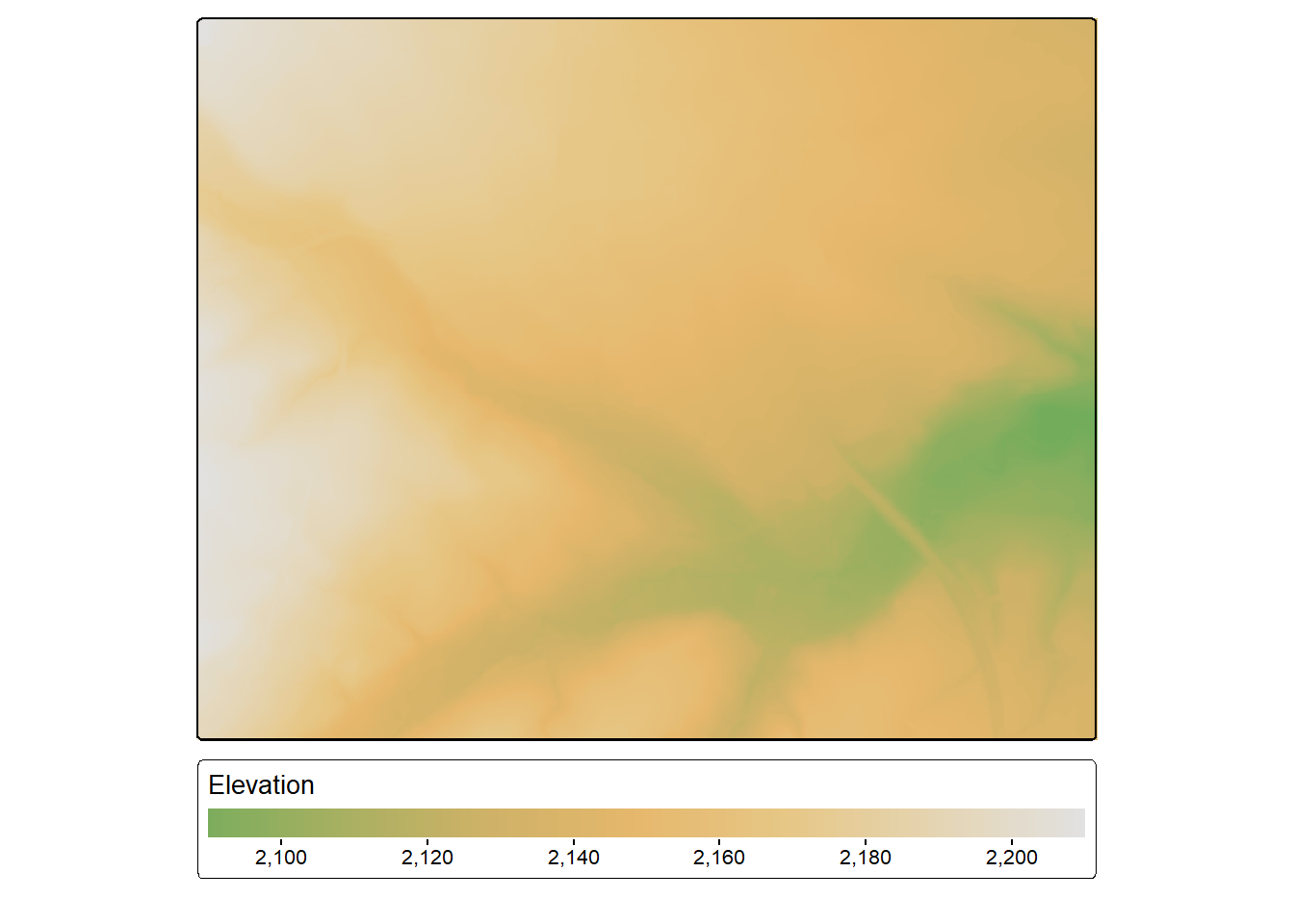
slp <- terrain(dtm,
               v ="slope",
               unit="radians")
asp <- terrain(dtm,
               v ="aspect",
               unit="radians")

hs <- shade(slp,
            asp,
            angle=45,
            direction=315)

tm_shape(hs)+
        tm_raster(col.scale = tm_scale_continuous(values="-brewer.greys"))+
  tm_shape(dtm)+
  tm_raster(col.scale = tm_scale_continuous(values="kovesi.linear_gow_65_90_c35"),
            col.legend = tm_legend(title="Elevation"),
            col_alpha=0.5)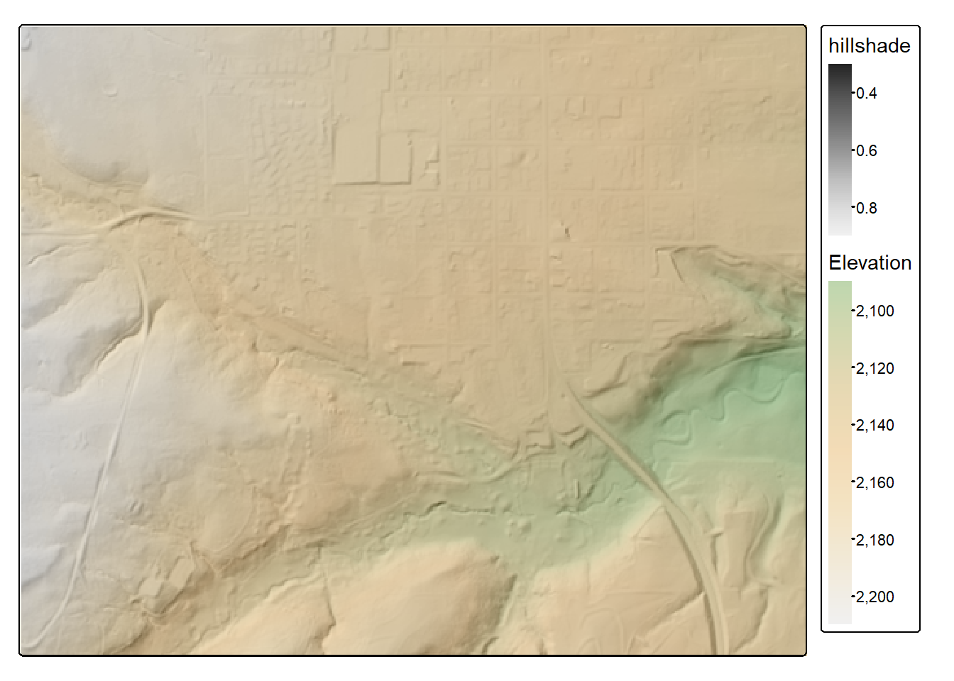
A DSM can be created with the rasterize_canopy() function. Algorithms available for creating a DSM are outlined in Chapter 7 of the lidR documentation. In our example, we use the pit-free algorithm as implemented with pitfree(). This algorithm uses a combination of Delaunay triangulation and pit removal/detection. We also fill empty cells using the mean value of neighboring cells and further smooth the result with a convolution filter. Both steps are implemented using the focal() function from terra.
dsm <- rasterize_canopy(lasAll,
                        res = 5,
                        pitfree(thresholds = c(0, 10, 20),
                                max_edge = c(0, 1.5)))

fill.na <- function(x, i=5) { if (is.na(x)[i]) { return(mean(x, na.rm = TRUE)) } else { return(x[i]) }}
w <- matrix(1, 3, 3)

dsm <- terra::focal(dsm,
                    w,
                    fun = fill.na)
dsm <- terra::focal(dsm,
                    w,
                    fun = mean,
                    na.rm = TRUE)
Once a DTM and DSM have been generated, an nDSM can be created by simply subtracting the DTM from the DSM using raster math. This product is generated below then visualized using tmap.
ndsm <- dsm - dtmtm_shape(ndsm)+
tm_raster(col.scale = tm_scale_intervals(n=7,
style="quantile",
values="yl_gn"),
col.legend = tm_legend(orientation= "landscape",
title="Height"))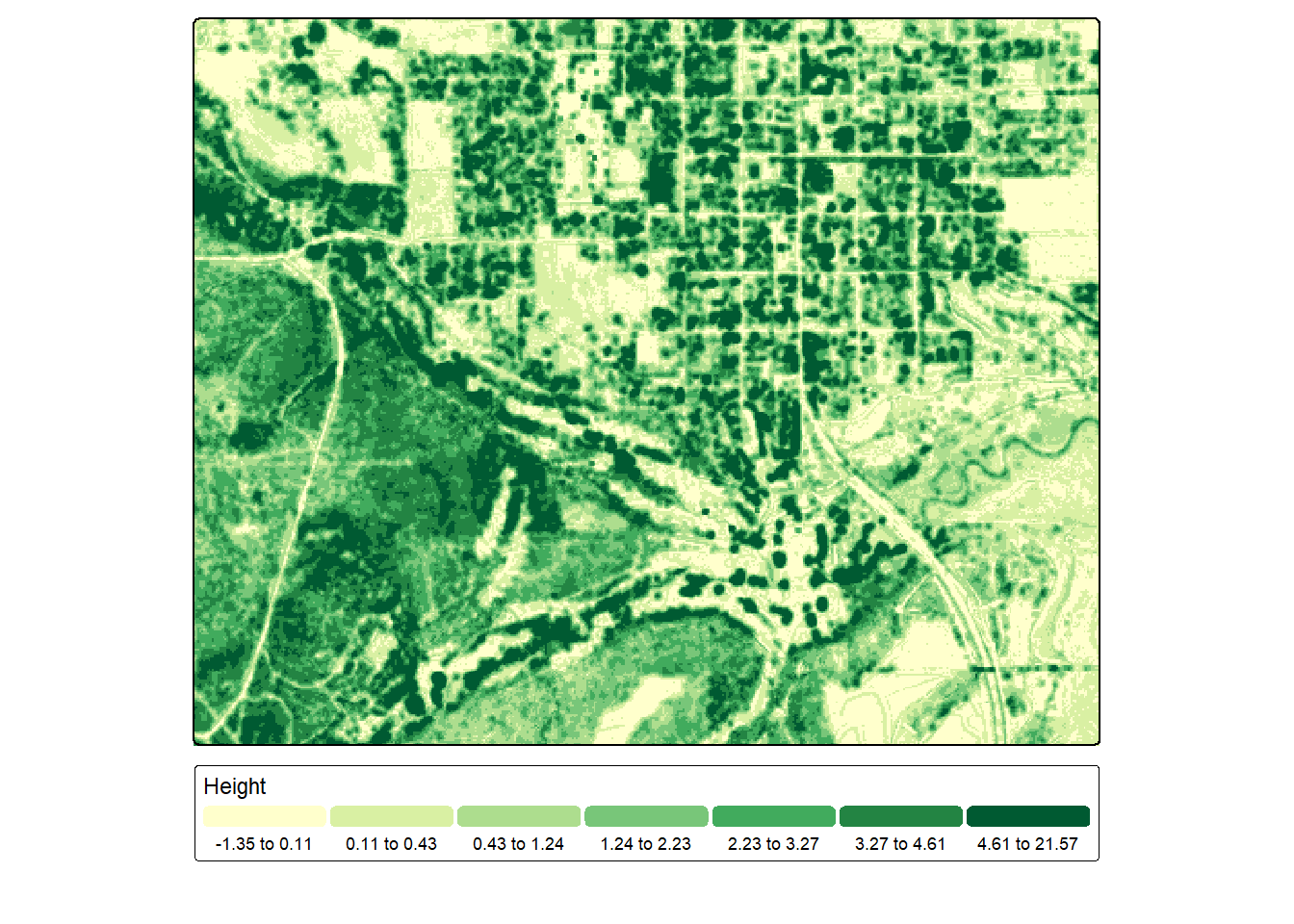
Lastly, it is often of value to normalize the z measurements to obtain height above the ground as opposed to the absolute elevation relative to a vertical datum. Conceptually, this is accomplished by subtracting the ground elevation at a points location from the point’s absolute elevation. In lidR, this can be accomplished using the ground classified data or a DTM. In our example, we use the ground classified data. Similar to generating a DTM, different interpolation methods can be used.
lasAllN <- normalize_height(lasAll, knnidw())Once the normalization is completed, we generate a histogram of the new z values to confirm that they represent height above ground as opposed to absolute elevation.
lasAllN@data |>
  ggplot(aes(x=Z))+
  geom_histogram()+
  scale_x_continuous(limits=c(-10, 50))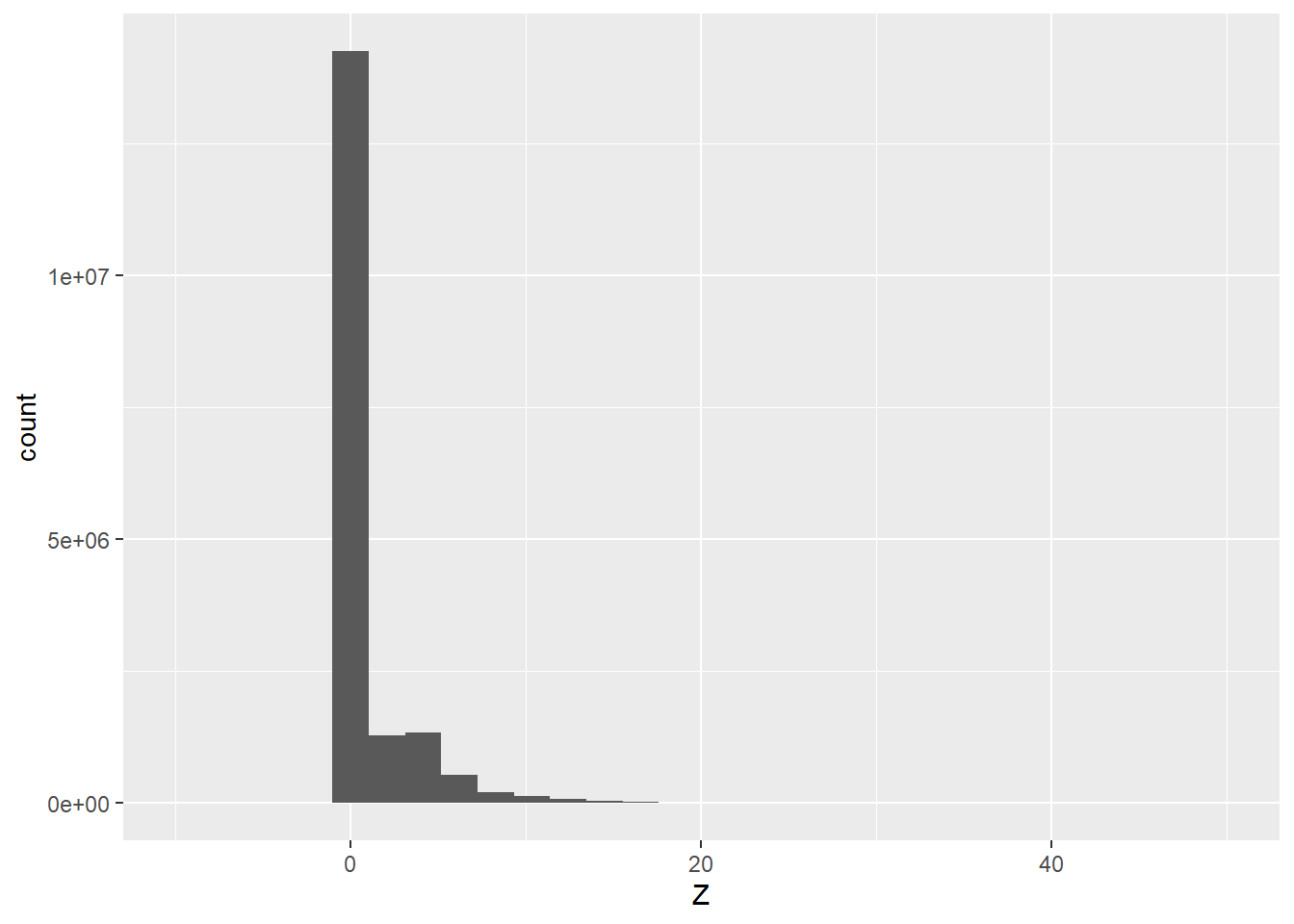
4.5 Summary Metrics
Point cloud data can be summarized at a variety of scales or aggregating units including:
- The entire point cloud
- Defined extents or plots
- At each raster cell location
- For each voxel in a 3D space
- For individual trees
Here, we demonstrate cloud-, plot-, and raster grid-level summarization since these are often most useful for spatial predictive mapping and modeling tasks.
4.5.1 Cloud-Level
The cloud_metrics() function is used to generate summary metrics for the entire point cloud. In our example, we use the ground normalized data and only consider non-ground points that are greater than 0.1 m from the ground. This is to avoid any unwanted near-ground noise or classification error.
In the first example, we calculate the mean height for this subset of returns, which is ~3.58 meters. In the next example, we generate a function to calculate the mean, median, standard deviation, and interquartile range (IQR) for the subset of points. This requires first defining the function then using it within cloud_metrics(). A list object is return, which is then converted to a data frame. Lastly, lidR includes pre-defined sets of metrics. We use the stdmetrics_z to obtain a variety of metrics as a list object, which is subsequently converted to a data frame.
lasAllN |> filter_poi(Classification != 2 & Z > .1) |>
  cloud_metrics(func= ~ mean(Z))
[1] 3.575112f <- function(z) {
list(
mnZ = mean(z),
mdZ = median(z),
sdZ = sd(z),
iqrZ = IQR(z))
}
cldMets <- lasAllN |> filter_poi(Classification != 2 & Z > .1) |>
cloud_metrics(func= ~ f(Z))
as.data.frame(do.call(cbind, cldMets)) |> gt()| mnZ | mdZ | sdZ | iqrZ |
|---|---|---|---|
| 3.575112 | 3.1 | 3.101621 | 3.4 |
cldMets <- lasAllN |> filter_poi(Classification != 2 & Z > .1) |>
  cloud_metrics(func= .stdmetrics_z)

as.data.frame(do.call(cbind, cldMets)) |> gt()| zmax | zmean | zsd | zskew | zkurt | zentropy | pzabovezmean | pzabove2 | zq5 | zq10 | zq15 | zq20 | zq25 | zq30 | zq35 | zq40 | zq45 | zq50 | zq55 | zq60 | zq65 | zq70 | zq75 | zq80 | zq85 | zq90 | zq95 | zpcum1 | zpcum2 | zpcum3 | zpcum4 | zpcum5 | zpcum6 | zpcum7 | zpcum8 | zpcum9 |
|---|---|---|---|---|---|---|---|---|---|---|---|---|---|---|---|---|---|---|---|---|---|---|---|---|---|---|---|---|---|---|---|---|---|---|---|
| 50.66 | 3.575112 | 3.101621 | 1.560419 | 6.548392 | 0.5663969 | 41.52842 | 67.44715 | 0.14 | 0.2 | 0.32 | 0.6 | 1.39 | 1.83 | 2.17 | 2.5 | 2.81 | 3.1 | 3.38 | 3.66 | 3.98 | 4.35 | 4.79 | 5.37 | 6.14 | 7.36 | 9.85 | 77.52156 | 95.39541 | 99.2106 | 99.97183 | 99.99865 | 99.99918 | 99.99958 | 99.9997 | 99.99989 |
4.5.2 Field Plot-Level
plot_metrics() allows for generate summary metrics using extents defined by a vector object. We make use of the 15 hypothetical field plot centers read in above, and metrics are calculated using all points in the subset that occur within a 30 m radius of the plot center or point location. This function returns an sf object, which we then display as a table after dropping the geometry.
One potential use of such a workflow would be to use the generated metrics along with ground measurements collected at the plot locations to build predictive models where the unit of analysis is individual plots. The goal would be to generate a model that can predict the field measurements using the point cloud characteristics as characterized by the set of summary metrics.
plotMets <- lasAllN |> filter_poi(Classification != 2 & Z > .1) |>
  plot_metrics(func = .stdmetrics_z,
               geometry = fPlts,
               radius = 30)

plotMets |>
  st_drop_geometry() |>
  gt() |>
  fmt_number(
    columns = everything(),
    decimals = 2,
use_seps = TRUE)| plotID | zmax | zmean | zsd | zskew | zkurt | zentropy | pzabovezmean | pzabove2 | zq5 | zq10 | zq15 | zq20 | zq25 | zq30 | zq35 | zq40 | zq45 | zq50 | zq55 | zq60 | zq65 | zq70 | zq75 | zq80 | zq85 | zq90 | zq95 | zpcum1 | zpcum2 | zpcum3 | zpcum4 | zpcum5 | zpcum6 | zpcum7 | zpcum8 | zpcum9 |
|---|---|---|---|---|---|---|---|---|---|---|---|---|---|---|---|---|---|---|---|---|---|---|---|---|---|---|---|---|---|---|---|---|---|---|---|---|
| 1.00 | 8.22 | 2.14 | 1.75 | 0.87 | 3.65 | 0.77 | 48.35 | 51.65 | 0.15 | 0.19 | 0.22 | 0.27 | 0.33 | 0.46 | 1.33 | 1.71 | 1.89 | 2.06 | 2.26 | 2.46 | 2.69 | 2.90 | 3.13 | 3.39 | 3.69 | 4.17 | 5.58 | 32.83 | 38.87 | 60.08 | 78.05 | 89.50 | 93.01 | 95.22 | 97.22 | 99.05 |
| 2.00 | 7.53 | 2.94 | 1.66 | 0.12 | 2.54 | 0.89 | 49.60 | 71.54 | 0.18 | 0.30 | 0.97 | 1.64 | 1.86 | 2.08 | 2.26 | 2.48 | 2.69 | 2.91 | 3.15 | 3.37 | 3.59 | 3.81 | 4.07 | 4.37 | 4.69 | 5.07 | 5.70 | 14.38 | 18.27 | 34.83 | 52.29 | 68.98 | 82.22 | 91.86 | 96.44 | 98.78 |
| 3.00 | 7.03 | 3.05 | 1.43 | −0.09 | 2.74 | 0.84 | 51.14 | 78.04 | 0.24 | 1.19 | 1.67 | 1.90 | 2.12 | 2.33 | 2.54 | 2.74 | 2.91 | 3.08 | 3.27 | 3.42 | 3.61 | 3.79 | 4.03 | 4.27 | 4.52 | 4.87 | 5.42 | 8.76 | 11.52 | 24.66 | 42.42 | 62.62 | 78.79 | 90.55 | 96.46 | 99.10 |
| 4.00 | 8.57 | 3.97 | 1.70 | −0.38 | 2.87 | 0.86 | 53.67 | 87.78 | 0.23 | 1.83 | 2.23 | 2.57 | 2.93 | 3.20 | 3.46 | 3.70 | 3.91 | 4.12 | 4.30 | 4.50 | 4.70 | 4.92 | 5.17 | 5.45 | 5.74 | 6.04 | 6.54 | 6.93 | 9.13 | 20.08 | 34.31 | 54.55 | 74.46 | 89.16 | 97.47 | 99.48 |
| 5.00 | 34.03 | 3.44 | 1.82 | 0.83 | 13.00 | 0.54 | 49.72 | 81.46 | 0.17 | 0.53 | 1.79 | 2.08 | 2.33 | 2.59 | 2.83 | 3.04 | 3.24 | 3.42 | 3.62 | 3.82 | 4.02 | 4.21 | 4.42 | 4.69 | 5.05 | 5.59 | 6.61 | 49.48 | 95.63 | 100.00 | 100.00 | 100.00 | 100.00 | 100.00 | 100.00 | 100.00 |
| 6.00 | 8.51 | 3.32 | 1.67 | −0.01 | 2.61 | 0.86 | 49.89 | 78.78 | 0.20 | 0.96 | 1.66 | 1.96 | 2.20 | 2.43 | 2.66 | 2.88 | 3.10 | 3.32 | 3.54 | 3.78 | 4.03 | 4.28 | 4.53 | 4.77 | 5.07 | 5.44 | 6.06 | 9.79 | 15.76 | 32.75 | 51.87 | 69.52 | 85.45 | 94.44 | 98.45 | 99.64 |
| 7.00 | 6.89 | 2.40 | 1.14 | 0.00 | 3.23 | 0.78 | 51.01 | 65.46 | 0.19 | 0.58 | 1.37 | 1.59 | 1.76 | 1.89 | 2.02 | 2.15 | 2.29 | 2.43 | 2.57 | 2.71 | 2.86 | 3.00 | 3.14 | 3.31 | 3.48 | 3.74 | 4.19 | 10.42 | 15.08 | 36.74 | 61.56 | 84.15 | 94.53 | 97.82 | 99.26 | 99.91 |
| 8.00 | 7.90 | 3.25 | 1.78 | −0.19 | 2.20 | 0.90 | 53.15 | 75.44 | 0.18 | 0.30 | 0.75 | 1.75 | 2.03 | 2.32 | 2.61 | 2.88 | 3.16 | 3.41 | 3.64 | 3.87 | 4.10 | 4.36 | 4.61 | 4.87 | 5.18 | 5.53 | 5.96 | 15.18 | 18.02 | 30.66 | 44.98 | 61.55 | 77.27 | 89.88 | 97.70 | 99.69 |
| 9.00 | 7.25 | 2.73 | 1.68 | 0.06 | 2.21 | 0.87 | 51.75 | 66.40 | 0.17 | 0.25 | 0.37 | 0.89 | 1.51 | 1.82 | 2.07 | 2.37 | 2.59 | 2.80 | 3.02 | 3.25 | 3.50 | 3.74 | 3.96 | 4.24 | 4.52 | 4.89 | 5.47 | 19.44 | 24.27 | 37.08 | 52.39 | 67.84 | 81.83 | 92.01 | 97.06 | 99.12 |
| 10.00 | 11.13 | 3.43 | 2.08 | 0.79 | 3.83 | 0.82 | 42.25 | 77.65 | 0.17 | 0.52 | 1.68 | 1.91 | 2.11 | 2.29 | 2.48 | 2.67 | 2.85 | 3.05 | 3.29 | 3.56 | 3.87 | 4.20 | 4.58 | 5.04 | 5.54 | 6.18 | 7.42 | 10.67 | 27.96 | 55.91 | 73.59 | 85.26 | 92.71 | 96.09 | 97.87 | 99.25 |
| 11.00 | 6.84 | 2.64 | 1.52 | −0.16 | 2.18 | 0.87 | 54.09 | 68.59 | 0.16 | 0.24 | 0.41 | 0.96 | 1.60 | 1.92 | 2.17 | 2.38 | 2.60 | 2.82 | 3.00 | 3.19 | 3.39 | 3.59 | 3.79 | 3.99 | 4.21 | 4.48 | 4.89 | 18.17 | 22.28 | 32.40 | 47.95 | 65.66 | 82.91 | 93.84 | 98.33 | 99.55 |
| 12.00 | 9.56 | 3.41 | 1.81 | 0.27 | 3.09 | 0.85 | 49.44 | 79.55 | 0.19 | 0.79 | 1.66 | 1.98 | 2.21 | 2.49 | 2.72 | 2.97 | 3.18 | 3.38 | 3.59 | 3.80 | 4.01 | 4.20 | 4.43 | 4.75 | 5.19 | 5.85 | 6.67 | 10.47 | 18.97 | 37.81 | 60.67 | 80.31 | 89.34 | 95.12 | 98.67 | 99.42 |
| 13.00 | 4.96 | 1.98 | 1.18 | −0.07 | 2.02 | 0.91 | 53.48 | 52.57 | 0.16 | 0.23 | 0.34 | 0.52 | 0.91 | 1.38 | 1.61 | 1.79 | 1.93 | 2.09 | 2.23 | 2.38 | 2.54 | 2.71 | 2.87 | 3.05 | 3.24 | 3.47 | 3.83 | 19.41 | 25.66 | 32.13 | 46.79 | 63.11 | 77.97 | 90.10 | 96.48 | 99.42 |
| 14.00 | 8.91 | 3.48 | 1.92 | −0.03 | 2.46 | 0.89 | 52.17 | 78.20 | 0.20 | 0.33 | 1.09 | 1.86 | 2.22 | 2.54 | 2.81 | 3.07 | 3.35 | 3.56 | 3.78 | 4.03 | 4.28 | 4.53 | 4.82 | 5.10 | 5.46 | 5.95 | 6.64 | 14.72 | 19.02 | 32.47 | 50.19 | 68.11 | 83.63 | 92.40 | 97.39 | 99.38 |
| 15.00 | 6.94 | 2.76 | 1.47 | 0.09 | 2.89 | 0.88 | 50.59 | 72.20 | 0.17 | 0.30 | 1.24 | 1.68 | 1.90 | 2.10 | 2.29 | 2.44 | 2.61 | 2.78 | 2.98 | 3.13 | 3.28 | 3.47 | 3.67 | 3.89 | 4.17 | 4.54 | 5.33 | 13.28 | 15.96 | 29.74 | 49.98 | 69.98 | 84.91 | 92.75 | 96.31 | 98.56 |
4.5.3 Pixel-Level
Pixel-level summarization is particularly useful for the types of spatial predictive mapping and modeling tasks discussed in this text since they allow us to generate wall-to-wall measures that can be used as predictor variables. These measures could be used as a feature space or combined with variables derived from other data sources, such as multispectral image bands, to enhance or improve the feature space.
Our first example below demonstrates calculating the standard deviation of the normalized heights for all points in 5 m raster cells using only returns that were not classified as ground points and were at least 0.1 m from the ground. Since cells with only ground returns will not contain any returns that meet this criteria, NA is returned at these cell locations, which are shaded gray in the map output using the value.na parameter within tm_scale_intervals().
sdZ <- lasAllN |> filter_poi(Classification != 2 & Z > .1) |>
  pixel_metrics(~sd(Z), 5)

tm_shape(sdZ)+
  tm_raster(col.scale = tm_scale_intervals(n=7,
                                           style="quantile",
                                           values="brewer.yl_or_rd",
                                           value.na="lightgray"),
            col.legend = tm_legend(orientation= "landscape",
                                   title="Z Standard Deviation"))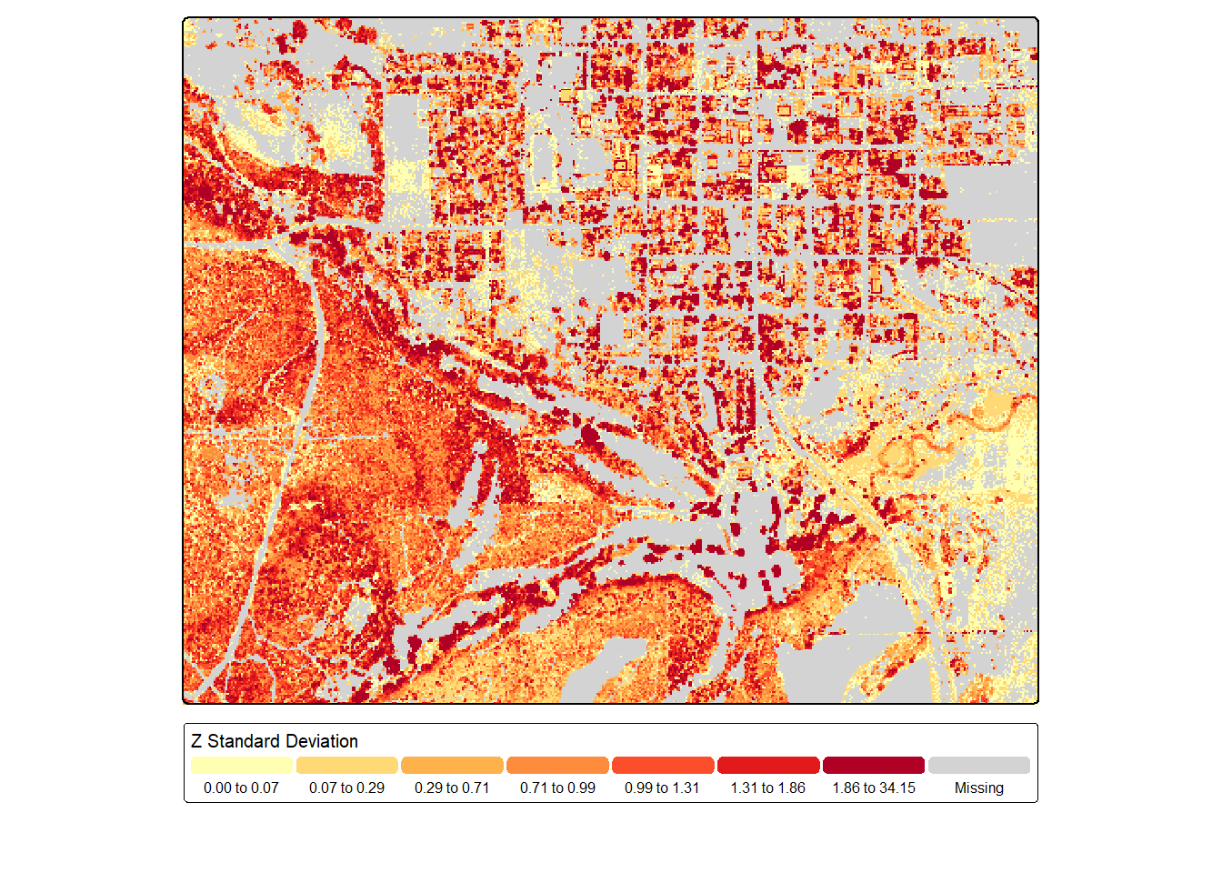
Next, we generated a first return intensity image by calculating the median intensity of all 1st returns (i.e., single or first of many) occurring within 5 m cells. Cells without first returns are coded as NA. We code these cells to zero using ifel() from terra based on the assumption that no returns were measured since all the energy was absorbed, as can happen over water bodies when using a near infrared (NIR) laser, which is the case for these data. Note that stripping pattern in the result, which is a flight line artifact. Despite this, patterns are still evident. For example, impervious surfaces and pavement are dark since they absorb a large proportion of the NIR laser pulse. Low vegetation appears brighter since it reflects a larger proportion of the NIR energy. Forests and vertical vegetation show a complex texture, generally resulting from the laser energy being split into multiple returns.
frstInt <- lasAllN |> filter_poi(ReturnNumber == 1) |>
  pixel_metrics(~median(as.double(Intensity)), 5)

frstInt <- ifel(is.na(frstInt), 0, frstInt)

tm_shape(frstInt)+
  tm_raster(col.scale = tm_scale_intervals(n=7,
                                           style="quantile",
                                           values="-brewer.greys"),
            col.legend = tm_legend(orientation= "landscape",
                                   title="First Resturn Intensity"))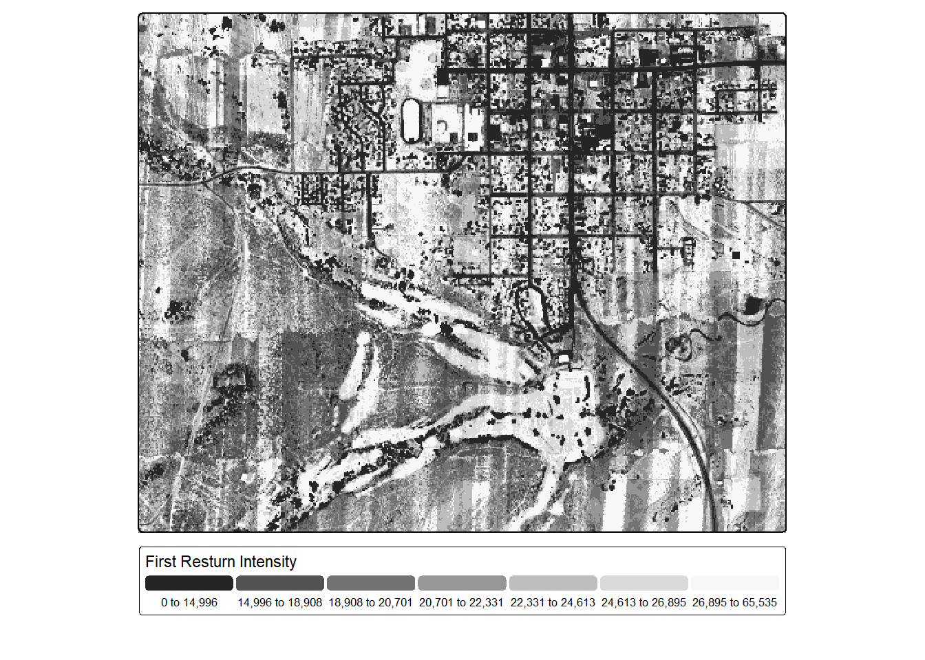
In the next code block, we count the number of non-ground returns that are greater than 0.1 m above the ground. Again, NA values are coded to zero since we assume these locations had no returns meeting the criteria. We generally see more returns over forests and wooded areas since single pulses are broken into multiple returns.
pntCnt <- lasAllN |> filter_poi(Classification != 2 & Z > .1) |>
  pixel_metrics(~length(Z), 5)

pntCnt <- ifel(is.na(pntCnt), 0, pntCnt)

tm_shape(pntCnt)+
  tm_raster(col.scale = tm_scale_intervals(n=7,
                                           style="quantile",
                                           values="met.tam",
                                           value.na="lightgray"),
            col.legend = tm_legend(orientation= "landscape",
                                   title="Point Count"))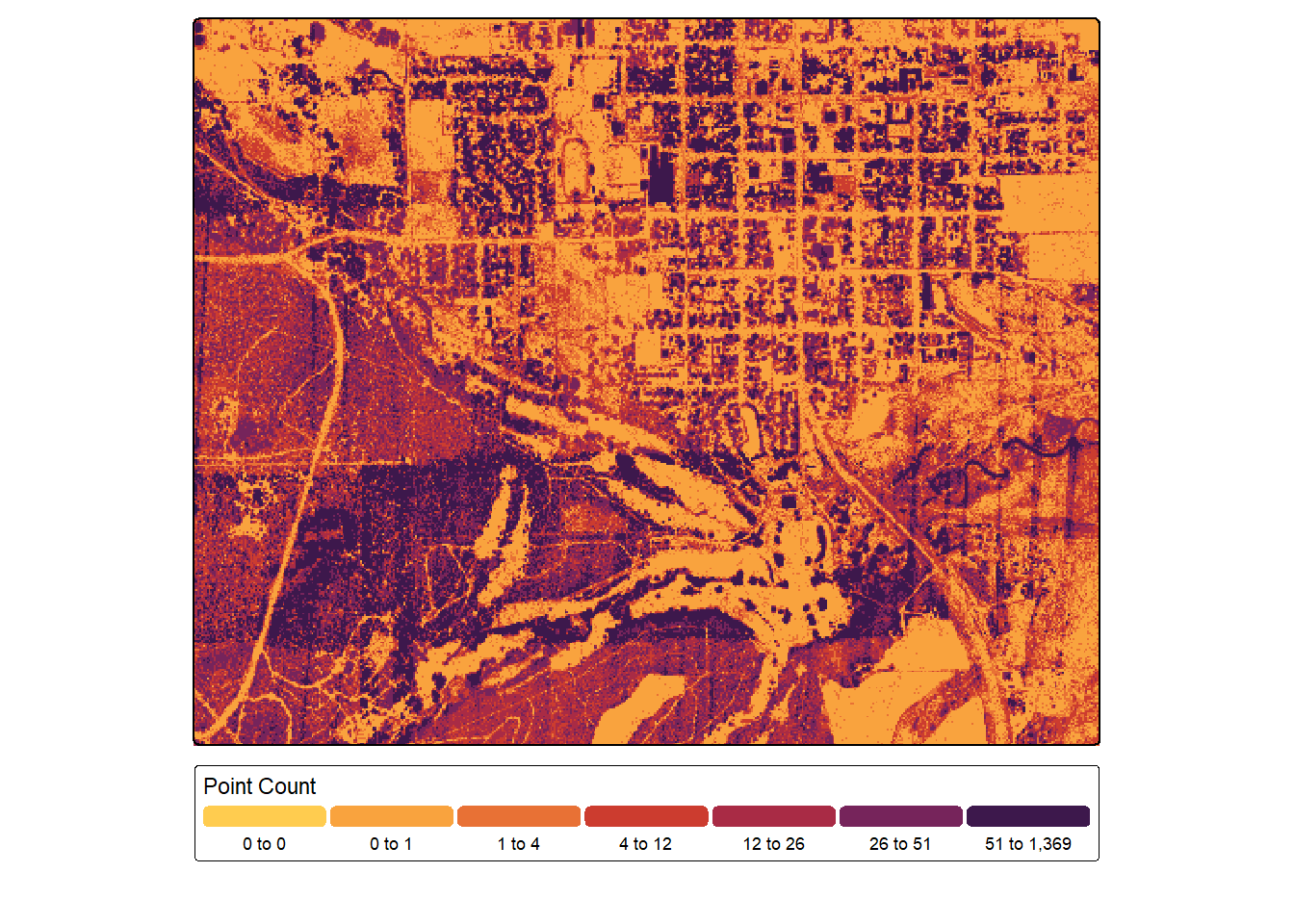
Lastly, we calculate the proportion of total returns that are not ground returns per cell. We can see some flight line artifacts but also correlation with forest or woodland areas.
pntCntG <- lasAllN |> filter_poi(Classification != 2 & Z <.1) |>
  pixel_metrics(~length(Z), 5)

pntCntG <- ifel(is.na(pntCntG), 0, pntCntG)

propNG <- (pntCnt-pntCntG)/(pntCnt+.001)

tm_shape(propNG)+
  tm_raster(col.scale = tm_scale_intervals(n=7,
                                           style="quantile",
                                           values="met.van_gogh3",
                                           value.na="lightgray"),
            col.legend = tm_legend(orientation= "landscape",
                                   title="Point Count"))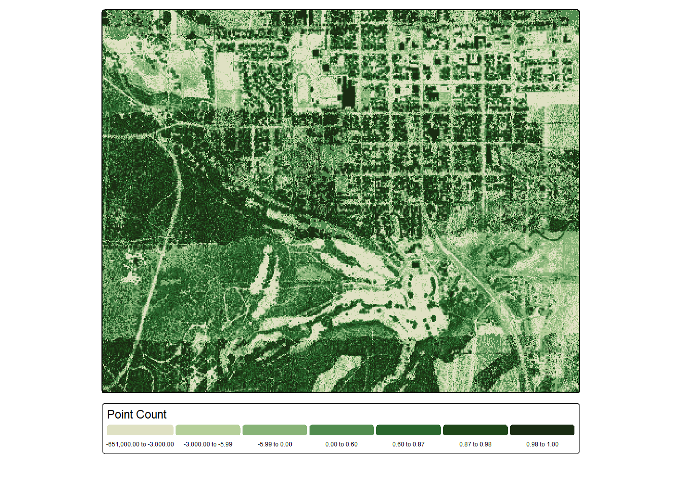
One complexity or challenges with raster-based summarization of point clouds is the wide variety of metrics that can be calculated. Selecting an optimal set of parameters to calculate can be a daunting task, and limited guidance may be available for your specific use case. We generally recommend selecting variables based on common sense. You should consider what information a variable captures and whether this information may be informative for your modeling or mapping problem. Visualizing variables, as demonstrated here, can also be informative.
4.6 LAS Catalog
Point clouds can be large, which complicates processing data over large extents and/or datasets with a high point density. To help scale processing and analysis to large data sets, lidR includes another means to represent point cloud data termed a LAS Catalog. This is similar to the concept of a LAS Dataset in the ESRI environment. A LAS Catalog can reference multiple files and process data using a tiling system so as not to overload available memory. Multiple tiles can be used collectively via virtual layers.
A LAS Catalog is created using readLAScatalog(). By providing a folder path, all .las or .laz files in the folder will be added to the catalog. Our example folder only contains one file.
lasCat <- readLAScatalog("gslrData/chpt4/data/")
summary(lasCat)
class : LAScatalog (v1.2 format 3)
extent : 643725.5, 646851.2, 4190956, 4193577 (xmin, xmax, ymin, ymax)
coord. ref. : WGS 84 / UTM zone 12N
area : 8.19 km²
points : 25.47 million points
density : 3.1 points/m²
density : 3 pulses/m²
num. files : 1
proc. opt. : buffer: 30 | chunk: 0
input opt. : select: * | filter:
output opt. : in memory | w2w guaranteed | merging enabled
drivers :
- Raster : format = GTiff NAflag = -999999
- stars : NA_value = -999999
- SpatRaster : overwrite = FALSE NAflag = -999999
- SpatVector : overwrite = FALSE
- LAS : no parameter
- Spatial : overwrite = FALSE
- sf : quiet = TRUE
- data.frame : no parameterUsing the plot() function, we can see that our catalog will be processed as a single tile since there is only one input file. We can set options for the LAS catalog to define the number of desired tiles or chunks. When there are multiple tiles or chunks, it is generally best to use a processing buffer to avoid edge effects and artifacts. In the second code block, we change the tile/chunk size to 1200 and set a 60 m buffer. We can confirm the change using plot().
plot(lasCat, chunk=TRUE)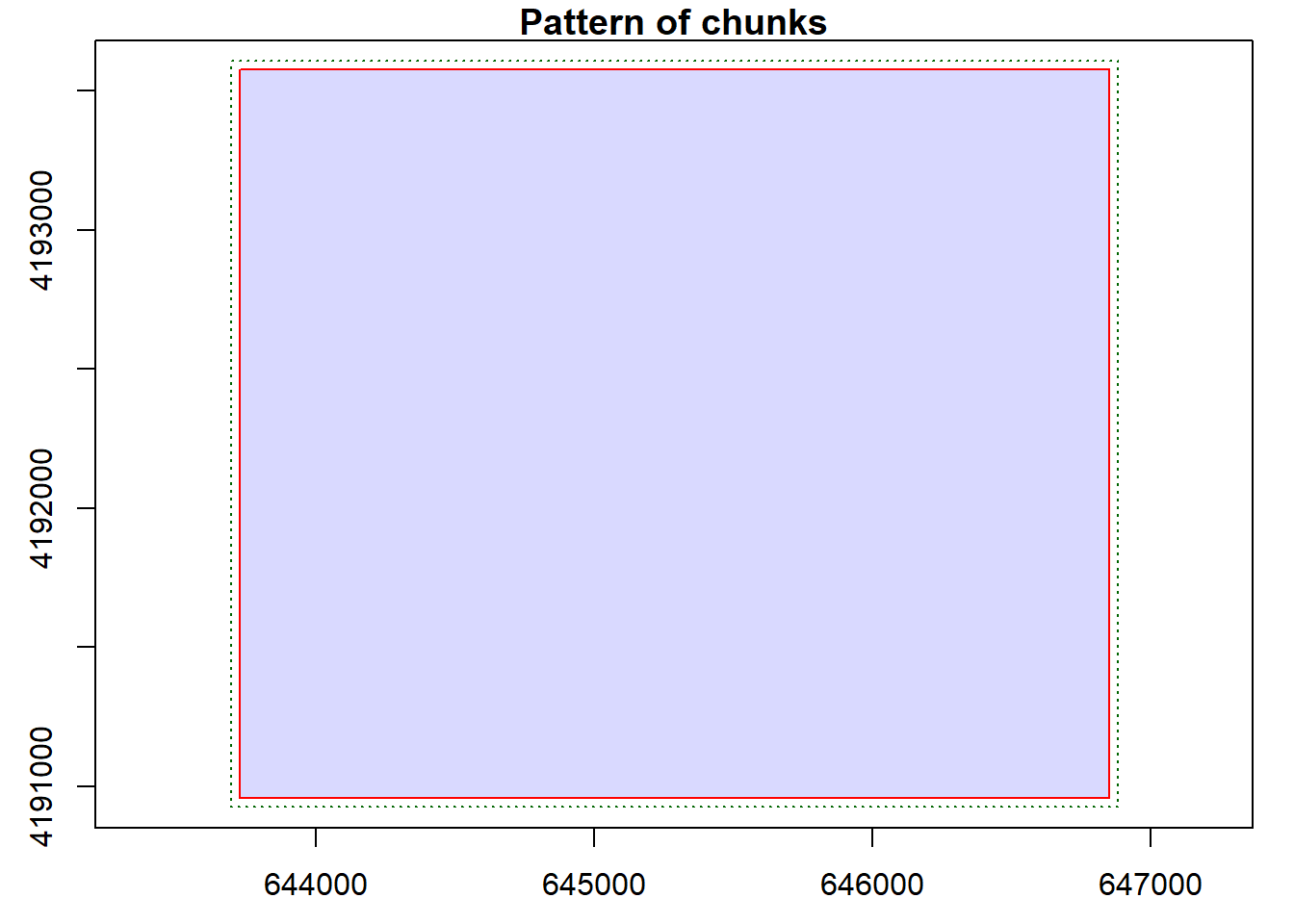
opt_chunk_size(lasCat) <- 1200
opt_chunk_buffer(lasCat) <- 60
plot(lasCat, chunk=TRUE)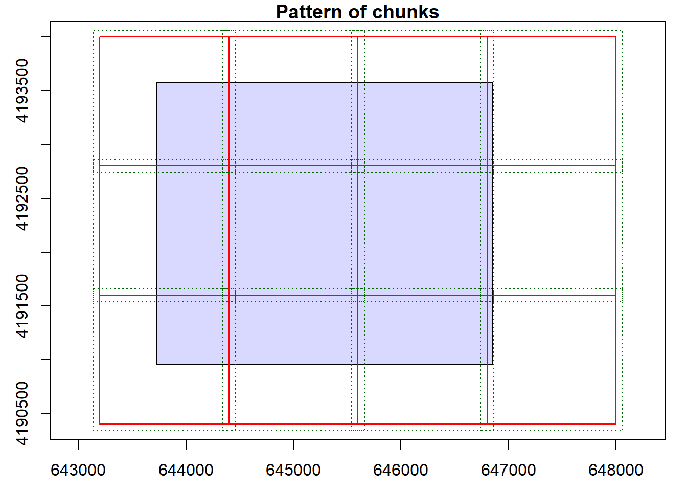
When a LAS catalog is processed, it is sometimes possible to store the results in memory. However, this is often unfeasible. To alleviate memory issues, results can be written to disk then referenced via a virtual file. This requires specifying a template for the file names for all files stored in a folder. We generally prefer to set up a temporary or scratch directory to store the files. In our example, the template indicates to name the tiles using the coordinates of their bottom-left corner.
In our specific example, we are using the pit free algorithm to generate an nDSM. The results for each tile are written into the scratch directory using the naming template we defined. They are referenced to a virtual raster which is associated with the dsm2 variable. We can even display this virtual file using tmap. Note that there are no obvious edge effects. This is due to the use of a processing buffer around each chunk.
opt_output_files(lasCat) <- "gslrData/chpt4/scratch/tile_{XLEFT}_{YBOTTOM}_dsm"
dsm2 <- rasterize_canopy(lasCat,
                         res = 5,
                         pitfree(thresholds = c(0, 10, 20),
                                 max_edge = c(0, 1.5)))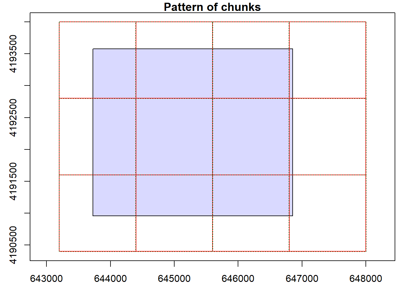
tm_shape(dsm2)+
  tm_raster(col.scale = tm_scale_intervals(n=7,
                                           style="quantile",
                                           values="yl_gn"),
            col.legend = tm_legend(orientation= "landscape",
                                   title="Elevation"))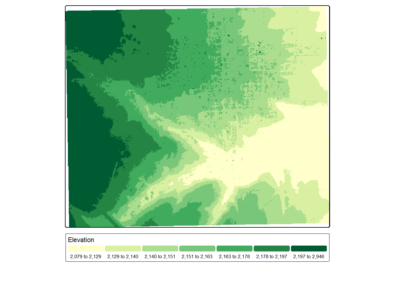
We can confirm that raster files have been written into the scratch directory by listing the files in the directory. Note that our naming convention was successfully applied.
list.files("glsrData/chpt4/scratch/")You can also apply filters to LAS Catalogs that will be honored when processes are applied to them. Below, we are changing which attributes are read in, reading only ground points, and selecting a subset based on a spatial extent. We also remove withheld data points.
opt_select(lasCat) <- "xyzicnr"
opt_filter(lasCat) <- "-drop_withheld -keep_class 2 -keep_xy 644077 4191186  646579 4193195"
This is a very general overview of LAS Catalogs. This structure is very powerful for processing large volumes of data, which is often necessary for applied mapping and modeling tasks. Chapter 15 and Chapter 16 of the lidR documentation offer more detailed discussions of LAS Catalogs.
4.7 Concluding Remarks
This is the last chapter devoted to data preprocessing. You should now have a decent understanding of how to work with and process raster data and point clouds using R and primarily the terra and lidR packages. We also more specifically discussed creating derivatives from multispectral imagery and DTMs, which we termed land surface parameters (LSPs). We discussed exploratory data analysis and preprocessing of tabulated data, with a specific focus on the recipes package. This package will be used throughout the next two sections of the text. The next chapter is the last chapter of Section 1 and explores accuracy assessment methods and metrics.
4.8 Questions
- What is a voxel?
- Explain how k-nearest neighbor inverse distance weighting works when interpolating a digital terrain model from classified ground points.
- Explain how the triangulated irregular network (TIN) method works for interpolating a digital terrain model from classified ground points.
- Compare lidar return intensity for vegetation, pavement, and water when using a near infrared laser.
- How does moisture content commonly impact return intensity when using a NIR laser?
- Conceptually explain how the cloth simulation function (CSF) works for performing a ground classification of lidar data.
- Conceptually explain how the pit-free algorithm works for generating a canopy height model (CHM) from a point cloud.
- Explain the entropy point cloud summarization metric.
4.9 Exercises
You have been provided with a single lidar point cloud (points.laz) in the exercise folder for the chapter. These data were provided by the United States Geological Survey (USGS) 3D Elevation (3DEP) and are for the area around Roaring Springs, Pennsylvania. Perform the following operations on the point cloud to generate derived products:
- Read in the data; you only need the “x”, “y”, “z”, “i” (return intensity), “c” (“classification”), and “r” (return number) attributes, and you can ignore withheld data points
- Use the
rasterize_terrain()function to convert the point cloud to a digital terrain model (DTM) at a 5 m spatial resolution; use theknnidw()function with 10 neighbors and a power of 2 - Visualize the generated DTM with tmap
- From the DTM, calculate, topographic slope, topographic aspect, and a hillshade
- Visualize the DTM with transparency over the hillshade using tmap
- Create a DSM using the
rasterize_canopy()function at a spatial resolution of 5 m; use thepitfree()function with the default settings - Create an nDSM by subtracting the DTM from the DSM
- Visualize the nDSM using tmap
- Create a 1st return intensity image at a 5 m spatial resolution using
pixel_metrics(); use the median value in each cell, and fill allNAcells with a value of0 - Visualize the 1st return intensity image with tmap
- Save the DTM, slope, aspect, hillshade, and nDSM raster grids to disk