import torch
import torchinfo
import torch.nn as nn
import torch.nn.functional as F10 Build a Convolutional Neural Network
10.1 Introduction
Now that you have an understanding of how CNNs work and the different layers that are used to construct them, you are ready to build a CNN architecture using PyTorch and by subclassing nn.Module. In this section, we will build a CNN. In the next section, we will prepare image data then train and assess a CNN. The last two sections focused on CNNs will explore some commonly used CNN architectures and how to implement transfer learning. In this module, you should focus on understanding how the CNN architecture is defined using PyTorch and not worry about the other components of training and implementing them.
A simple CNN for scene labeling is conceptualized in Figure 10.1. The architecture consists of two components. The first component is a series of convolutional blocks, each of which applies 2D convolution, batch normalization, a ReLU activation, and max pooling. With each block, the number of feature maps increases while the height and width of the feature maps are halved by the max pooling operation. The second component is a fully connected network. The feature maps generated by the last convolutional block are flattened to a 1D array and passed through fully connected layers, and the final layer outputs a logit for each class, which can be converted to class probabilities using a softmax activation. The CNN defined in this chapter follows this general structure.
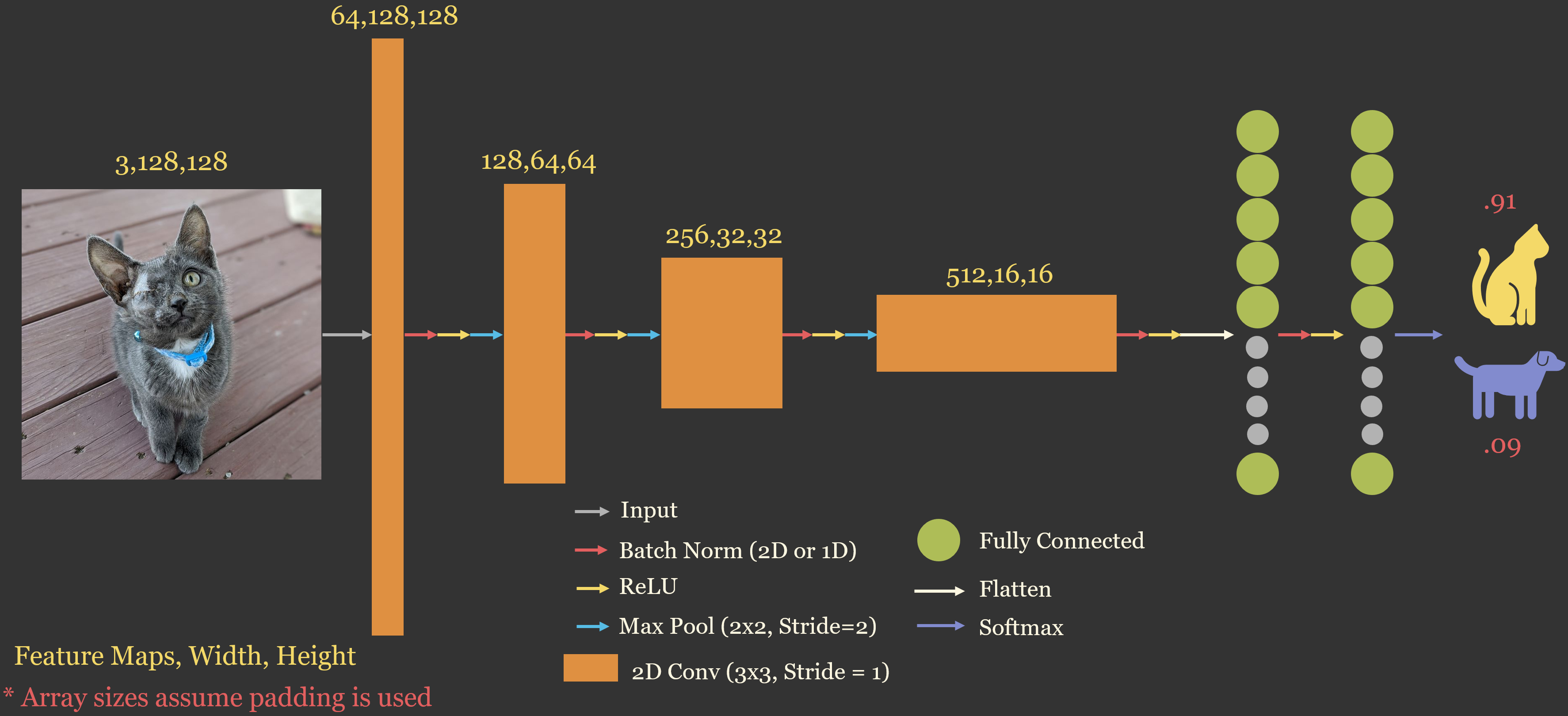
I first import the required packages. Next, I define the device. If a GPU is available, it is used. If one is not available, the CPU is used. Note that training a CNN using a CPU can be very slow. So, if you plan to explore CNNs further, you need to have access to a CUDA-enabled GPU.
device = torch.device("cuda:0" if torch.cuda.is_available() else "cpu")print(device)cuda:010.2 Define Architecture
My goal is to build a CNN that allows the user to define the number of classes, number of input channels, number of feature maps in each convolution layer, and the number of nodes in each fully connected layer. The CNN will have the following general architecture.
A total of 4 2D convolutional layers.
After each convolutional layer, batch normalization will be applied followed by a rectified linear unit (ReLU) activation.
After the convolutional component of the model, the resulting array will be flattened.
The flatten array, or 1D vector, will be passed through 3 fully connected layers.
After each of the first 2 fully connected layers, batch normalization will be applied followed by a ReLU activation.
After the final fully connected layer, no batch normalization or activation will be applied, and raw logits will be delivered.
I will need to know the height and width of the array after the final max pooling operation is applied. So, I write a simple helper function that allows me to calculate the height and width after the final max pooling operation if provided with the original input size and the number of convolution blocks. The function simply divides the original size by two in a loop in which the number of loop iterations is equivalent to the number of convolution blocks and associated max pooling operations.
I test this simple function using an original input size of 128x128 and 4 convolution blocks. Given these inputs, the final height and width of the tensor after all 4 max pooling operations are applied will be 8x8 (128x128 –> 64x64 –> 32x32 –> 16x16 –> 8x8).
def getDim(inDim, numBlks):
  x = inDim
  for i in range(1,numBlks+1,1):
    x = x/2
return int(x)getDim(128, 4)8I first define my CNN without using nn.Sequential(). Later, I will replicate this process using nn.Sequential(). This is accomplished by subclassing nn.Module. Here is a walk through of the process.
Begin by subclassing
nn.Module(). I usesuper().__init__()inside of the__init__()constructor method and also define all input parameters.I then define all of the required layers within the
__init__()constructor method. A total of 4nn.Conv2d()operations are defined. Note that the first one will accept the number of input channels and output the first provided output channel size. Each subsequentnn.Conv2d()layer requires that the in_channels parameter be equal to the out_channels parameter of the prior convolution operation. Within allnn.Conv2d()blocks, I use a kernel size of (3x3) and a padding of 1. This will result in an output height and width that is the same as the input height and width for that specificnn.Conv2d()layer.I then define associated
nn.BatchNorm2d()layers for eachnn.Conv2d()layer. The number of features parameter is equivalent to the output channel size of the associatednn.Conv2d()layer.I define an
nn.ReLU()and annn.MaxPool2d()layer. These only need defined once since they have the same settings each time they are called. For max pooling, a kernel size of 2x2 is used with a stride of 2. This will result in decreasing the array size by half in the spatial dimensions.I then define the fully connected layers. The first fully connected layer will have an input size equal to the number of output channels from the last convolution layer multiplied by the height and width of the tensor following the last max pooling application. All subsequent layers require that the number of input features be equivalent to the number of output features from the prior fully connected layer. The last fully connected layer must have an output size equal to the number of classes being differentiated.
I define batch normalization layers to accompany the first and second fully connected layers. Since these are fully connected layers, I used
nn.BatchNorm1d()as opposed tonn.BatchNorm2d(). The number of features parameter must be equivalent to the number of output features from the associated fully connected layer.In the forward method, how the input data will be passed through the network is defined. Within each convolution block the sequence is 2D Convolution –> Batch Normalization –> ReLU Activation –> Max Pooling.
Once the data have been passed through the convolutional component of the architecture, they are flattened to a 1D tensor using
view().The flatten tensor is then passed through the fully connected layers. Note that no batch normalization or activation function is applied after the last fully connected layer.
I am not applying a softmax activation. As a result, the logits will be returned as opposed to probabilities.
class myCNN(nn.Module):
  def __init__(self, nCls, inChn, outChn, fcChn, lastDim):
    super().__init__()
    self.nCls = nCls
    self.inChn = inChn
    self.outChn = outChn
    self.fcChn = fcChn
    self.lastDim = lastDim

    self.conv1 = nn.Conv2d(in_channels=inChn, out_channels=outChn[0], kernel_size=3, padding=1)
    self.conv2 = nn.Conv2d(in_channels=outChn[0], out_channels=outChn[1], kernel_size=(3,3), padding=1)
    self.conv3 = nn.Conv2d(in_channels=outChn[1], out_channels=outChn[2], kernel_size=(3,3), padding=1)
    self.conv4 = nn.Conv2d(in_channels=outChn[2], out_channels=outChn[3], kernel_size=(3,3), padding=1)

    self.bn1 = nn.BatchNorm2d(outChn[0])
    self.bn2 = nn.BatchNorm2d(outChn[1])
    self.bn3 = nn.BatchNorm2d(outChn[2])
    self.bn4 = nn.BatchNorm2d(outChn[3])

    self.relu = nn.ReLU()
    self.pool = nn.MaxPool2d(kernel_size=(2,2),stride=2)

    self.fc1 = nn.Linear(lastDim*lastDim*outChn[3], fcChn[0])
    self.fc2 = nn.Linear(fcChn[0],  fcChn[1])
    self.fc3 = nn.Linear(fcChn[1], nCls)

    self.bnfc1 = nn.BatchNorm1d(fcChn[0])
    self.bnfc2 = nn.BatchNorm1d(fcChn[1])

  def forward(self, x):
    x = self.pool(self.relu(self.bn1(self.conv1(x))))
    x = self.pool(self.relu(self.bn2(self.conv2(x))))
    x = self.pool(self.relu(self.bn3(self.conv3(x))))
    x = self.pool(self.relu(self.bn4(self.conv4(x))))
    x = x.view(-1, self.lastDim*self.lastDim*self.outChn[3])
    x = self.relu(self.bnfc1(self.fc1(x)))
    x = self.relu(self.bnfc2(self.fc2(x)))
    x = self.fc3(x)
    return x
Once the CNN architecture is defined, I instantiate an instance of the subclass. Here, I must define the number of classes to differentiate, the number of input channels, a list of number of kernels to learn in each convolution block that must be the same length as the number of convolution blocks, the number of features for the first and second fully connected layers as a list, and the height and width of the tensor following the last max pooling operation. This is required to calculate the length of the flattened array prior to feeding it through the fully connected layers. This is calculated using the helper function I defined above.
The model is then moved to the device using the to() method.
model = myCNN(nCls=10,
              inChn=3,
              outChn=[10,20,30,40],
              fcChn=[268,512],
              lastDim=getDim(128,4)).to(device)
The torchinfo package allows for summarizing a neural network. The summary() function accepts a model and an associated input tensor shape. It provides a summary including the layers being used, the shape of the output of each layer, and the number of parameters. It also lists the number of total parameters, the number of trainable parameters, and the number of non-trainable parameters. The size of the model in regards to memory consumption is also estimated.
In the example below, I have performed the summarization using an array size of (12,3,128,128). This represents a mini-batch containing 12 images. Each image has 3 bands and a height and width of 128 pixels. Note that the spatial dimension of the array is halved after every max pooling operation. Most of the trainable parameters are associated with the kernel weights and biases and fully connected layer weights and biases. However, there are also some trainable parameters associated with the batch normalization layers (i.e., gain and shift parameters). The ReLU and max pooling layers have no trainable parameters.
Lastly, note that the there are no non-trainable parameters. This is because none of the layers have been frozen. We will discuss freezing components of an architecture in later modules.
torchinfo.summary(model, (12,3,128,128))==========================================================================================
Layer (type:depth-idx) Output Shape Param #
==========================================================================================
myCNN [12, 10] --
├─Conv2d: 1-1 [12, 10, 128, 128] 280
├─BatchNorm2d: 1-2 [12, 10, 128, 128] 20
├─ReLU: 1-3 [12, 10, 128, 128] --
├─MaxPool2d: 1-4 [12, 10, 64, 64] --
├─Conv2d: 1-5 [12, 20, 64, 64] 1,820
├─BatchNorm2d: 1-6 [12, 20, 64, 64] 40
├─ReLU: 1-7 [12, 20, 64, 64] --
├─MaxPool2d: 1-8 [12, 20, 32, 32] --
├─Conv2d: 1-9 [12, 30, 32, 32] 5,430
├─BatchNorm2d: 1-10 [12, 30, 32, 32] 60
├─ReLU: 1-11 [12, 30, 32, 32] --
├─MaxPool2d: 1-12 [12, 30, 16, 16] --
├─Conv2d: 1-13 [12, 40, 16, 16] 10,840
├─BatchNorm2d: 1-14 [12, 40, 16, 16] 80
├─ReLU: 1-15 [12, 40, 16, 16] --
├─MaxPool2d: 1-16 [12, 40, 8, 8] --
├─Linear: 1-17 [12, 268] 686,348
├─BatchNorm1d: 1-18 [12, 268] 536
├─ReLU: 1-19 [12, 268] --
├─Linear: 1-20 [12, 512] 137,728
├─BatchNorm1d: 1-21 [12, 512] 1,024
├─ReLU: 1-22 [12, 512] --
├─Linear: 1-23 [12, 10] 5,130
==========================================================================================
Total params: 849,336
Trainable params: 849,336
Non-trainable params: 0
Total mult-adds (Units.MEGABYTES): 254.50
==========================================================================================
Input size (MB): 2.36
Forward/backward pass size (MB): 55.20
Params size (MB): 3.40
Estimated Total Size (MB): 60.96
==========================================================================================10.3 Define Architecture using nn.Sequential()
In the code block below, I have defined the same network as above but now making use of nn.Sequential(). After instantiating an instance of the model and using the summary function from torchsummary, you can see that the resulting model is the same as the one defined above. So, either method is valid for defining the model architecture. Whether or not you want to use nn.Sequential() comes down to personal preference; however, it can simplify the code in many cases. I generally prefer to use nn.Sequential() as I find the code more readable.
class myCNNSeq(nn.Module):
  def __init__(self, nCls, inChn, outChn, fcChn, lastDim):
    super().__init__()
    self.nCls = nCls
    self.inChn = inChn
    self.outChn = outChn
    self.fcChn = fcChn
    self.lastDim = lastDim

    self.cnnLyrs = nn.Sequential(
        nn.Conv2d(in_channels=inChn, out_channels=outChn[0], kernel_size=(3,3), padding=1),
        nn.BatchNorm2d(outChn[0]),
        nn.ReLU(inplace=True),
        nn.MaxPool2d(2,2),
        nn.Conv2d(in_channels=outChn[0], out_channels=outChn[1], kernel_size=(3,3), padding=1),
        nn.BatchNorm2d(outChn[1]),
        nn.ReLU(inplace=True),
        nn.MaxPool2d(2,2),
        nn.Conv2d(in_channels=outChn[1], out_channels=outChn[2], kernel_size=(3,3), padding=1),
        nn.BatchNorm2d(outChn[2]),
        nn.ReLU(inplace=True),
        nn.MaxPool2d(2,2),
        nn.Conv2d(in_channels=outChn[2], out_channels=outChn[3], kernel_size=(3,3), padding=1),
        nn.BatchNorm2d(outChn[3]),
        nn.ReLU(inplace=True),
        nn.MaxPool2d(2,2)
    )

    self.fcLyrs = nn.Sequential(
        nn.Linear(lastDim*lastDim*outChn[3], fcChn[0]),
        nn.BatchNorm1d(fcChn[0]),
        nn.ReLU(inplace=True),
        nn.Linear(fcChn[0], fcChn[1]),
        nn.BatchNorm1d(fcChn[1]),
        nn.ReLU(inplace=True),
        nn.Linear(fcChn[1], nCls)
    )

  def forward(self,x):
    x = self.cnnLyrs(x)
    x = x.view(-1, self.lastDim*self.lastDim*self.outChn[3])
    x = self.fcLyrs(x)
    return x
model2 = myCNNSeq(nCls=10,
inChn=3,
outChn=[10,20,30,40],
fcChn=[268,512],
lastDim=getDim(128,4)).to(device)torchinfo.summary(model2, (12,3,128,128))==========================================================================================
Layer (type:depth-idx) Output Shape Param #
==========================================================================================
myCNNSeq [12, 10] --
├─Sequential: 1-1 [12, 40, 8, 8] --
│ └─Conv2d: 2-1 [12, 10, 128, 128] 280
│ └─BatchNorm2d: 2-2 [12, 10, 128, 128] 20
│ └─ReLU: 2-3 [12, 10, 128, 128] --
│ └─MaxPool2d: 2-4 [12, 10, 64, 64] --
│ └─Conv2d: 2-5 [12, 20, 64, 64] 1,820
│ └─BatchNorm2d: 2-6 [12, 20, 64, 64] 40
│ └─ReLU: 2-7 [12, 20, 64, 64] --
│ └─MaxPool2d: 2-8 [12, 20, 32, 32] --
│ └─Conv2d: 2-9 [12, 30, 32, 32] 5,430
│ └─BatchNorm2d: 2-10 [12, 30, 32, 32] 60
│ └─ReLU: 2-11 [12, 30, 32, 32] --
│ └─MaxPool2d: 2-12 [12, 30, 16, 16] --
│ └─Conv2d: 2-13 [12, 40, 16, 16] 10,840
│ └─BatchNorm2d: 2-14 [12, 40, 16, 16] 80
│ └─ReLU: 2-15 [12, 40, 16, 16] --
│ └─MaxPool2d: 2-16 [12, 40, 8, 8] --
├─Sequential: 1-2 [12, 10] --
│ └─Linear: 2-17 [12, 268] 686,348
│ └─BatchNorm1d: 2-18 [12, 268] 536
│ └─ReLU: 2-19 [12, 268] --
│ └─Linear: 2-20 [12, 512] 137,728
│ └─BatchNorm1d: 2-21 [12, 512] 1,024
│ └─ReLU: 2-22 [12, 512] --
│ └─Linear: 2-23 [12, 10] 5,130
==========================================================================================
Total params: 849,336
Trainable params: 849,336
Non-trainable params: 0
Total mult-adds (Units.MEGABYTES): 254.50
==========================================================================================
Input size (MB): 2.36
Forward/backward pass size (MB): 55.20
Params size (MB): 3.40
Estimated Total Size (MB): 60.96
==========================================================================================10.4 Wrapping the CNN in a LightningModule
In Chapter 8, we wrapped a fully connected architecture in a LightningModule so that it could be trained using PyTorch Lightning. Since the LightningModule stores the architecture as an attribute, the same LightningModule can be used to train any scene classification architecture, including the CNN defined in this chapter, without any changes to the training code. Below, I define a general LitClassifier class that accepts an instantiated architecture, the number of classes, and a learning rate. This is the same as the LightningModule from Chapter 8 except that the architecture is provided as an argument as opposed to being defined inside of the class. We will use this class to train CNNs in Chapter 11, Chapter 12, and Chapter 13.
Since the architecture is an nn.Module object as opposed to a simple value, I exclude it from the saved hyperparameters using self.save_hyperparameters(ignore=["model"]). As a result, the architecture must be provided again when the model is loaded from a checkpoint.
import lightning as L
import torchmetrics as tm

class LitClassifier(L.LightningModule):
    def __init__(self, model, nCls, lr=1e-3):
        super().__init__()
        self.save_hyperparameters(ignore=["model"])
        self.model = model
        self.criterion = nn.CrossEntropyLoss()
        self.lr = lr

        metrics = tm.MetricCollection({
            "acc": tm.Accuracy(task="multiclass", num_classes=nCls),
            "f1": tm.F1Score(task="multiclass", num_classes=nCls, average="macro"),
            "kappa": tm.CohenKappa(task="multiclass", num_classes=nCls),
        })
        self.train_metrics = metrics.clone(prefix="train_")
        self.val_metrics = metrics.clone(prefix="val_")
        self.test_metrics = metrics.clone(prefix="test_")

    def forward(self, x):
        return self.model(x)

    def _shared_step(self, batch, metrics, stage):
        x, y = batch
        logits = self(x)
        loss = self.criterion(logits, y)
        metrics.update(logits, y)
        self.log(f"{stage}_loss", loss, on_step=False, on_epoch=True, prog_bar=True)
        self.log_dict(metrics, on_step=False, on_epoch=True, prog_bar=(stage == "val"))
        return loss

    def training_step(self, batch, batch_idx):
        return self._shared_step(batch, self.train_metrics, "train")

    def validation_step(self, batch, batch_idx):
        self._shared_step(batch, self.val_metrics, "val")

    def test_step(self, batch, batch_idx):
        self._shared_step(batch, self.test_metrics, "test")

    def predict_step(self, batch, batch_idx):
        x = batch[0] if isinstance(batch, (list, tuple)) else batch
        return torch.softmax(self(x), dim=1)

    def configure_optimizers(self):
        return torch.optim.AdamW(self.parameters(), lr=self.lr)
Note that the training, validation, and test steps are nearly identical, so I have defined a _shared_step() method that is called by each of them. The leading underscore is a Python convention indicating that the method is meant for internal use within the class. The predict_step() method returns class probabilities, which can be converted to “hard” predictions using argmax().
To demonstrate, I wrap the CNN defined above in a LitClassifier and summarize it using Lightning’s ModelSummary utility. By default, the Lightning summary lists the submodules and the number of parameters in each. Setting the example_input_array attribute to a tensor of the expected shape allows the summary to also report the input and output shapes of each submodule, similar to torchinfo. The max_depth argument controls how many levels of nested submodules are displayed.
from lightning.pytorch.utilities.model_summary import ModelSummary

litCNN = LitClassifier(model=myCNN(nCls=10, inChn=3, outChn=[10, 20, 30, 40],
                                   fcChn=[256, 512], lastDim=getDim(128, 4)),
                       nCls=10, lr=1e-3)
litCNN.example_input_array = torch.zeros(12, 3, 128, 128)
print(ModelSummary(litCNN, max_depth=2))
Which summary tool should you use? Both report the number of trainable and non-trainable parameters and the estimated model size. torchinfo provides a more detailed, layer-by-layer summary, including the output shape of every layer, which is very useful when building and debugging architectures, as we do throughout this text. Lightning’s summary is printed automatically at the start of training and is convenient for confirming that the expected architecture and parameters are being trained. I generally use torchinfo when designing an architecture and rely on Lightning’s summary during training.
10.5 Concluding Remarks
You now know how to build a CNN architecture using PyTorch and by subclassing the nn.Module class. This architecture was constructed using a small set of layer types: 2D convolution, 2D batch normalization, ReLU activation function, max pooling, fully connected layers, and 1D batch normalization. Further, the model was generalized so that the user could provide inputs with varying shapes and define the number of classes that will be differentiated, output number of learned kernels for each convolution layer, and intermediate sizes of the fully connected layers.
We also wrapped the architecture in a general LightningModule that can be used to train any scene classification architecture. Now, we are ready to train a CNN.
10.6 Questions
- Describe the sequence of operations applied within each convolutional block of the CNN built in this chapter.
- An input image with a height and width of 128 pixels passes through four convolutional blocks, each of which ends with max pooling using a 2x2 window and a stride of 2. What will the height and width of the resulting tensor be? If the last convolutional layer generates 64 feature maps, how many inputs will the first fully connected layer require?
- Why must the tensor be flattened between the convolutional and fully connected components of a CNN for scene labeling? How was this accomplished in this chapter?
- Why is
nn.BatchNorm2d()used after the convolutional layers whilenn.BatchNorm1d()is used after the fully connected layers? - How many trainable parameters (weights and biases) are associated with a 2D convolutional layer that accepts 3 input channels and generates 16 feature maps using a 3x3 kernel? How many trainable parameters are associated with the batch normalization layer that follows it?
- Which of the layer types used in this chapter have trainable parameters, and which do not?
- Compare the model summaries provided by torchinfo and PyTorch Lightning’s
ModelSummary. In what situation would a model have non-trainable parameters? Why can the same LightningModule be used to train different scene classification architectures? - Why is a softmax activation not included at the end of the CNN architecture defined in this chapter?
10.7 Exercises
Exercise 10.1: Define a CNN Architecture
Introduction
The goal of this exercise is to build a CNN architecture for a scene classification task. You will train this architecture in Exercise 11.1.
Deliverables
- A Quarto (.qmd) file containing all required code and answers to the questions and discussion prompts, and the HTML webpage rendered from it
Data
This exercise makes use of the PatternNet dataset and the DataSet and DataLoaders that you created in Exercise 5.1. See that exercise for a description of the dataset.
Background Questions
Question 1: Explain the purpose of the stride parameter when configuring a convolutional layer.
Question 2: Explain the purpose of the padding parameter when configuring a convolutional layer.
Question 3: Why is it necessary to flatten the tensor between the convolutional and fully connected components of a CNN architecture for scene classification?
Question 4: Describe a means to decrease the size of tensors in the spatial dimensions other than using pooling layers.
Tasks
Task 1: Define a CNN architecture by subclassing nn.Module. The architecture should meet the following criteria:
- Accepts a mini-batch of tensors with a shape of (mini-batch, channels, height, width) where the channels dimension has a length of 3 (red, green, and blue) and the height and width dimensions have a length of 256.
- Has a total of 4 convolutional layers that generate 4, 8, 16, and 32 feature maps, respectively. Each convolutional layer should use a 3×3 kernel, a stride of 1, and a padding of 1.
- Each convolutional layer should be followed by a batch normalization layer, a ReLU activation function, and a max pooling operation. All max pooling operations should use a kernel size of 2×2 and a stride of 2.
- The fully connected component of the architecture should include 3 fully connected layers. The first fully connected layer must accept an input size equal to the length of the flattened array produced at the end of the convolutional component of the architecture and generate 128 outputs. The second layer should accept 128 inputs and generate 256 outputs. The last layer should accept 256 inputs and generate 38 outputs, one for each differentiated class.
- Include batch normalization layers and a ReLU activation function after the first two fully connected layers.
- The model should output 38 raw logits. Do not rescale the logits using a softmax activation within the model.
Task 2: Instantiate an instance of the model.
Task 3: Print a model summary using torchinfo. List the number of trainable parameters associated with:
- Weights in the convolutional kernels
- Biases in the convolutional kernels
- Gain and shift parameters in all batch normalization layers
- Weights in the fully connected layers
- Biases in the fully connected layers
How many total trainable parameters are included in the model? What is the estimated file size of the model if saved to disk?
Task 4: Using the DataLoaders created in Exercise 5.1, predict a mini-batch of training data with the model to confirm that it accepts data in the correct shape.