import torch
import torch.nn as nn
import torch.nn.functional as F
import torchvision
from torchinfo import summary

device = torch.device("cuda:0" if torch.cuda.is_available() else "cpu")24 ConvNeXt
24.1 Introduction
Around 2020, transformer architectures, which were originally developed for natural language processing, began to outperform CNNs on image classification benchmarks. The Vision Transformer (ViT) and the Swin Transformer, in particular, led many researchers to question whether convolution was still the best choice for computer vision. We explore transformers in Chapter 25. In response, Liu et al. (2022) asked a different question: how much of the transformers’ advantage was due to self-attention, and how much was due to the many other design decisions and training techniques that came with them? Starting from a standard ResNet-50, they “modernized” the architecture step by step, adopting the design choices of transformers but keeping convolution, and evaluated the impact of each change. The result, ConvNeXt, is a pure CNN that matched or exceeded the performance of the Swin Transformer while retaining the simplicity and efficiency of CNNs.
Liu, Z., Mao, H., Wu, C.Y., Feichtenhofer, C., Darrell, T. and Xie, S., 2022. “A ConvNet for the 2020s.” In Proceedings of the IEEE/CVF Conference on Computer Vision and Pattern Recognition (pp. 11976-11986).
In this chapter, I explain the design of ConvNeXt, build a ConvNeXt block from scratch, use the pre-trained ConvNeXt architectures provided by torchvision, and demonstrate how ConvNeXt blocks can be integrated into a UNet for semantic segmentation, using the ConvNeXt UNet implemented in our terrainseg package as an example. We will also introduce ConvNeXt V2, which is closely tied to the fully convolutional masked autoencoder pre-training method explored in Chapter 27.
24.2 Modernizing a CNN
Liu et al. made the following changes, many of which are inspired by the Swin Transformer:
- Modern training recipe: training for more epochs with the AdamW optimizer, extensive data augmentation (e.g., Mixup, CutMix, and RandAugment), and regularization (e.g., stochastic depth and label smoothing, which we discussed in Chapter 7). This alone substantially improved the accuracy of the original ResNet-50, highlighting that some of the transformers’ advantage came from how they were trained.
- Stage compute ratio: the number of blocks in each of the four stages was changed from (3, 4, 6, 3) in ResNet-50 to (3, 3, 9, 3), placing more computation in the third stage.
- “Patchify” stem: the ResNet stem, a 7x7 convolution with a stride of 2 followed by max pooling, was replaced with a 4x4 convolution with a stride of 4. This splits the image into non-overlapping 4x4 patches, similar to how a ViT splits an image into patches.
- Depthwise convolution: the 3x3 convolutions were replaced with depthwise convolutions, as used in MobileNetV2 (Chapter 12), which process each channel separately. Depthwise convolution is similar to the weighted sum operation in self-attention, which mixes information spatially within each channel, while 1x1 convolutions mix information across channels. The width of the network was increased to compensate for the reduced computation.
- Inverted bottleneck: like the MLP block in a transformer and the inverted residual block in MobileNetV2, each block expands the number of channels by a factor of 4 and then projects them back.
- Large kernels: the depthwise convolution was moved to the beginning of the block, and its kernel size was increased to 7x7. Self-attention in the Swin Transformer operates over 7x7 windows, and larger kernels capture more spatial context.
- Micro design: ReLU was replaced with GELU (Chapter 7); fewer activation functions and normalization layers were used (only one of each per block, as in a transformer); batch normalization was replaced with layer normalization; and separate downsampling layers (2x2 convolutions with a stride of 2) were added between stages.
24.2.1 The ConvNeXt Block
The resulting ConvNeXt block consists of:
- A 7x7 depthwise convolution
- Layer normalization
- A 1x1 convolution that expands the number of channels by a factor of 4
- A GELU activation
- A 1x1 convolution that projects the number of channels back to the input size
- Layer scale: a learnable per-channel multiplier, initialized to a very small value (e.g., 1e-6), which allows each block to start close to the identity and stabilizes the training of deep networks
- Stochastic depth (or drop path): during training, the entire residual branch is randomly skipped for some samples, which acts as a regularizer. The probability of skipping increases with depth.
- A residual connection that adds the block’s input to its output
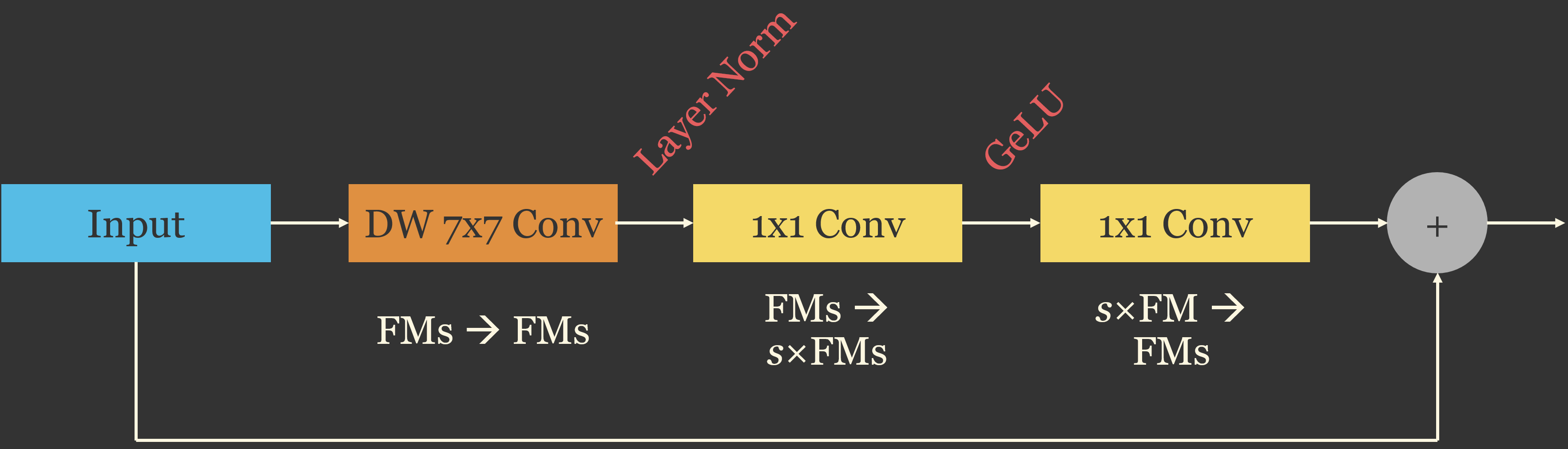
The ConvNeXt block is conceptualized in Figure 24.1. Note that the design follows an inverted bottleneck: the 1x1 convolutions expand the number of feature maps by a factor of s (4 by default) and then project them back to the original number, similar to the MLP in a transformer block. Only a single normalization layer and a single activation function are used in each block. Layer scale and stochastic depth are not pictured.
24.2.2 Layer Normalization
Batch normalization normalizes each channel using statistics calculated across the samples in the mini-batch and the spatial dimensions. Layer normalization normalizes each sample independently, using statistics calculated across the channels at each pixel location. Since it does not depend on the other samples in the mini-batch, layer normalization behaves the same during training and inference and is not affected by the mini-batch size. This is especially useful for geospatial semantic segmentation, where large image chips often limit the mini-batch size to a few samples, which makes batch normalization statistics unreliable. Group normalization is a compromise that normalizes each sample using statistics calculated across groups of channels.
PyTorch’s nn.LayerNorm normalizes over the last dimension(s) of a tensor, so it expects channels-last data. For channels-first image tensors, the class below normalizes over the channel dimension at each pixel location.
class LayerNorm2d(nn.Module):
    """Layer normalization over the channel dimension for (N, C, H, W) tensors."""
    def __init__(self, nChn, eps=1e-6):
        super().__init__()
        self.weight = nn.Parameter(torch.ones(nChn))
        self.bias = nn.Parameter(torch.zeros(nChn))
        self.eps = eps

    def forward(self, x):
        mean = x.mean(dim=1, keepdim=True)
        var = (x - mean).pow(2).mean(dim=1, keepdim=True)
        x = (x - mean) / torch.sqrt(var + self.eps)
        return x * self.weight[:, None, None] + self.bias[:, None, None]
The ConvNeXt block can now be defined. As in the original implementation, the 1x1 convolutions are implemented as fully connected layers applied to channels-last data, which is equivalent and slightly faster; the tensor is permuted before and after.
class ConvNeXtBlock(nn.Module):
    def __init__(self, dim, mlpRatio=4, dropPath=0.0, layerScaleInit=1e-6):
        super().__init__()
        self.dwconv = nn.Conv2d(dim, dim, kernel_size=7, padding=3, groups=dim)  # depthwise
        self.norm = nn.LayerNorm(dim, eps=1e-6)                                   # channels-last
        self.pwconv1 = nn.Linear(dim, mlpRatio * dim)                             # expand
        self.act = nn.GELU()
        self.pwconv2 = nn.Linear(mlpRatio * dim, dim)                             # project
        self.gamma = nn.Parameter(layerScaleInit * torch.ones(dim))               # layer scale
        self.dropPath = dropPath

    def forward(self, x):
        shortcut = x
        x = self.dwconv(x)
        x = x.permute(0, 2, 3, 1)            # (N, C, H, W) -> (N, H, W, C)
        x = self.pwconv2(self.act(self.pwconv1(self.norm(x))))
        x = (self.gamma * x).permute(0, 3, 1, 2)
        if self.training and self.dropPath > 0:   # stochastic depth: drop the branch per sample
            keep = torch.rand(x.shape[0], 1, 1, 1, device=x.device) >= self.dropPath
            x = x * keep / (1 - self.dropPath)
        return shortcut + x
blk = ConvNeXtBlock(96)
x = torch.rand(4, 96, 64, 64)
print(blk(x).shape)
summary(blk, (4, 96, 64, 64))Note how few parameters the block has relative to a standard double convolution block with the same number of channels, since the 7x7 convolution is depthwise. Most of the parameters are in the two 1x1 convolutions.
24.3 ConvNeXt in torchvision
torchvision provides four sizes of ConvNeXt, which differ in their widths and depths, along with ImageNet pre-trained weights: ConvNeXt-T (Tiny, ~28 million parameters), ConvNeXt-S (Small), ConvNeXt-B (Base), and ConvNeXt-L (Large). ConvNeXt-T has four stages with 96, 192, 384, and 768 channels and (3, 3, 9, 3) blocks. The features attribute contains the stem, the four stages, and the downsampling layers between them, and the classifier attribute contains the classification head.
modelCNX = torchvision.models.convnext_tiny(weights="DEFAULT").to(device)
print(summary(modelCNX, (12, 3, 224, 224), depth=2))
for i, m in enumerate(modelCNX.features):
    print(i, type(m).__name__)
As with the other torchvision architectures in Chapter 12, the stem can be replaced to accept a different number of input channels and the final layer of the classifier can be replaced to output the desired number of classes. The model can then be trained using the LitClassifier LightningModule from Chapter 10. Note that the patchify stem reduces the spatial dimensions by a factor of 4 and the total reduction is a factor of 32, so ConvNeXt is better suited to larger chips than the 64x64 EuroSAT chips.
def initialize_convnext(nChn, nCls, weights="DEFAULT"):
    model = torchvision.models.convnext_tiny(weights=weights)
    model.features[0][0] = nn.Conv2d(nChn, 96, kernel_size=4, stride=4)
    model.classifier[2] = nn.Linear(model.classifier[2].in_features, nCls)
    return model

summary(initialize_convnext(nChn=10, nCls=10), (12, 10, 128, 128))
24.4 ConvNeXt V2 and Global Response Normalization
ConvNeXt V2 (Woo et al., 2023) made two contributions. The first is the fully convolutional masked autoencoder (FCMAE), a self-supervised pre-training method for ConvNeXt, which is the topic of Chapter 27. The second is global response normalization (GRN), a layer added to the ConvNeXt block after the GELU activation. The authors found that, when ConvNeXt is pre-trained with FCMAE, many feature maps become redundant or inactive, which they called feature collapse. GRN encourages competition between channels: it calculates the global magnitude (L2 norm) of each feature map, normalizes these magnitudes relative to their mean across channels, and uses the result to rescale each feature map. Channels with relatively large responses are emphasized, and the diversity of the features increases. With GRN, layer scale is no longer needed.
Woo, S., Debnath, S., Hu, R., Chen, X., Liu, Z., Kweon, I.S. and Xie, S., 2023. “ConvNeXt V2: Co-designing and scaling ConvNets with masked autoencoders.” In Proceedings of the IEEE/CVF Conference on Computer Vision and Pattern Recognition (pp. 16133-16142).
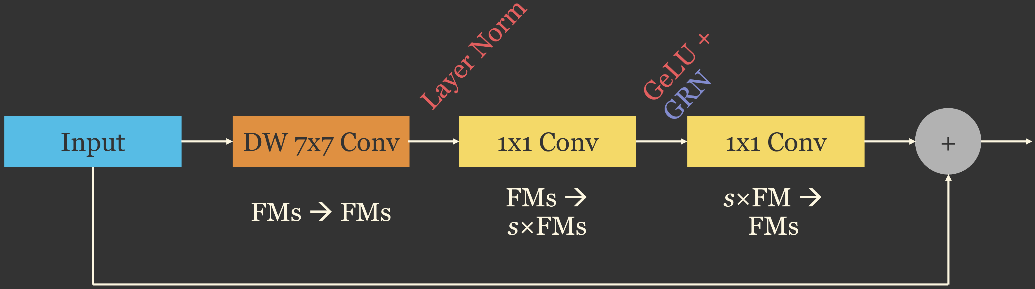
The ConvNeXt V2 block is conceptualized in Figure 24.2. The only differences from the original ConvNeXt block are the addition of GRN after the GELU activation and the removal of layer scale. The GRN module, which is conceptualized in Figure 24.3, consists of three steps. First, the global magnitude of each channel is aggregated by calculating its L2 norm across all spatial locations. Second, each channel’s magnitude is normalized by dividing it by the mean magnitude of all channels, which measures the relative importance of the channel. Third, the features are calibrated by multiplying them by the normalized values, scaling and shifting the result using learnable parameters (\(\gamma\) and \(\beta\)), and adding the input using a residual connection. Since \(\gamma\) and \(\beta\) are initialized to 0, the GRN module initially passes its input through unchanged.

class GRN(nn.Module):
    """Global response normalization for channels-last (N, H, W, C) tensors."""
    def __init__(self, dim):
        super().__init__()
        self.gamma = nn.Parameter(torch.zeros(1, 1, 1, dim))
        self.beta = nn.Parameter(torch.zeros(1, 1, 1, dim))

    def forward(self, x):
        gx = torch.norm(x, p=2, dim=(1, 2), keepdim=True)        # global magnitude per channel
        nx = gx / (gx.mean(dim=-1, keepdim=True) + 1e-6)           # relative to the mean of all channels
        return self.gamma * (x * nx) + self.beta + x

class ConvNeXtV2Block(nn.Module):
    def __init__(self, dim, mlpRatio=4, dropPath=0.0):
        super().__init__()
        self.dwconv = nn.Conv2d(dim, dim, kernel_size=7, padding=3, groups=dim)
        self.norm = nn.LayerNorm(dim, eps=1e-6)
        self.pwconv1 = nn.Linear(dim, mlpRatio * dim)
        self.act = nn.GELU()
        self.grn = GRN(mlpRatio * dim)
        self.pwconv2 = nn.Linear(mlpRatio * dim, dim)
        self.dropPath = dropPath

    def forward(self, x):
        shortcut = x
        x = self.dwconv(x).permute(0, 2, 3, 1)
        x = self.pwconv2(self.grn(self.act(self.pwconv1(self.norm(x))))).permute(0, 3, 1, 2)
        if self.training and self.dropPath > 0:
            keep = torch.rand(x.shape[0], 1, 1, 1, device=x.device) >= self.dropPath
            x = x * keep / (1 - self.dropPath)
        return shortcut + x
ConvNeXt V2 is not currently included in torchvision, but pre-trained ConvNeXt V2 models are available through the timm package (e.g., timm.create_model("convnextv2_tiny", pretrained=True)).
24.5 Integrating ConvNeXt Blocks into UNet
ConvNeXt blocks can be used in a UNet in several ways: (1) a pre-trained ConvNeXt can serve as the encoder, as we did with VGGNet, ResNet, and MobileNetV2 in Chapter 17; (2) ConvNeXt blocks can replace the double convolution blocks in a UNet trained from scratch; or (3) both. The Segmentation Models package supports option 1 through its interface to timm encoders (e.g., encoder_name="tu-convnext_tiny").
Here, I demonstrate option 2. Its design is as follows:
- Stem: a 3x3 convolution, followed by group normalization and GELU, maps the input to the first stage width at full resolution. Unlike the patchify stem used for classification, this maintains the full resolution so that a skip connection can be provided at the original resolution.
- Encoder: four stages. Each stage applies a sequence of ConvNeXt blocks at a fixed width, saves the output for the skip connection, and then reduces the spatial dimensions by half using a 2x2 convolution with a stride of 2, which also increases the number of channels. This replaces max pooling, as in ConvNeXt.
- Bottleneck: a sequence of ConvNeXt blocks at the lowest resolution.
- Decoder: four stages. Each upsamples by a factor of 2 (using bilinear interpolation followed by a 1x1 convolution, or a transpose convolution), optionally projects the skip features using a 1x1 convolution with group normalization and GELU, filters the skip features using an attention gate (Chapter 18), concatenates them with the upsampled features, and applies a residual double convolution block that uses group normalization and GELU.
- Head: a 1x1 convolution that outputs the class logits.
Group normalization is used in the stem and decoder, and layer normalization is used in the ConvNeXt blocks, so the architecture does not depend on the mini-batch size. Below, I define the encoder and decoder stages and assemble the model. Note that the attention gate in this design operates at the same resolution as the skip features, since the decoder features are upsampled before being used as the gating signal; this differs slightly from the attention gate used in Chapter 18.
def gnGroups(nChn, groups=8):
    g = min(groups, nChn)
    while nChn % g:
        g -= 1
    return g

class DownStage(nn.Module):
    def __init__(self, inDim, outDim, depth=2, mlpRatio=4):
        super().__init__()
        self.blocks = nn.Sequential(*[ConvNeXtBlock(inDim, mlpRatio) for _ in range(depth)])
        self.down = nn.Conv2d(inDim, outDim, kernel_size=2, stride=2)

    def forward(self, x):
        skip = self.blocks(x)
        return skip, self.down(skip)

class AttentionGateSame(nn.Module):
    def __init__(self, xChn, gChn):
        super().__init__()
        inter = max(1, xChn // 2)
        self.theta = nn.Conv2d(xChn, inter, kernel_size=1, bias=False)
        self.phi = nn.Conv2d(gChn, inter, kernel_size=1, bias=False)
        self.psi = nn.Sequential(nn.ReLU(), nn.Conv2d(inter, 1, kernel_size=1), nn.Sigmoid())

    def forward(self, x, g):
        return x * self.psi(self.theta(x) + self.phi(g))

class ResDoubleConvGN(nn.Module):
    def __init__(self, inChn, outChn, groups=8):
        super().__init__()
        g = gnGroups(outChn, groups)
        self.f = nn.Sequential(
            nn.Conv2d(inChn, outChn, 3, padding=1, bias=False), nn.GroupNorm(g, outChn), nn.GELU(),
            nn.Conv2d(outChn, outChn, 3, padding=1, bias=False), nn.GroupNorm(g, outChn), nn.GELU())
        self.proj = nn.Identity() if inChn == outChn else nn.Sequential(
            nn.Conv2d(inChn, outChn, 1, bias=False), nn.GroupNorm(g, outChn))

    def forward(self, x):
        return self.f(x) + self.proj(x)

class UpStage(nn.Module):
    def __init__(self, inDim, skipDim, outDim, groups=8):
        super().__init__()
        self.up = nn.Conv2d(inDim, outDim, kernel_size=1, bias=False)
        self.skipProj = nn.Sequential(nn.Conv2d(skipDim, outDim, 1, bias=False),
                                      nn.GroupNorm(gnGroups(outDim, groups), outDim), nn.GELU())
        self.attn = AttentionGateSame(outDim, outDim)
        self.conv = ResDoubleConvGN(2 * outDim, outDim, groups)

    def forward(self, x, skip):
        x = self.up(F.interpolate(x, scale_factor=2, mode="bilinear", align_corners=False))
        skip = self.attn(self.skipProj(skip), x)
        return self.conv(torch.cat([skip, x], dim=1))

class ConvNeXtUNet(nn.Module):
    def __init__(self, inChn=3, nCls=2, features=(64, 128, 256, 512, 1024),
                 encDepths=(2, 2, 2, 2), btnDepth=2, mlpRatio=4, groups=8):
        super().__init__()
        c1, c2, c3, c4, c5 = features
        self.stem = nn.Sequential(nn.Conv2d(inChn, c1, 3, padding=1, bias=False),
                                  nn.GroupNorm(gnGroups(c1, groups), c1), nn.GELU())
        self.down = nn.ModuleList([DownStage(a, b, d, mlpRatio)
                                   for a, b, d in zip((c1, c2, c3, c4), (c2, c3, c4, c5), encDepths)])
        self.bottleneck = nn.Sequential(*[ConvNeXtBlock(c5, mlpRatio) for _ in range(btnDepth)])
        self.up = nn.ModuleList([UpStage(a, s, s, groups)
                                 for a, s in zip((c5, c4, c3, c2), (c4, c3, c2, c1))])
        self.head = nn.Conv2d(c1, nCls, kernel_size=1)

    def forward(self, x):
        x = self.stem(x)
        skips = []
        for stage in self.down:
            skip, x = stage(x)
            skips.append(skip)
        x = self.bottleneck(x)
        for stage, skip in zip(self.up, skips[::-1]):
            x = stage(x, skip)
        return self.head(x)
model = ConvNeXtUNet(inChn=3, nCls=5, features=(32, 64, 128, 256, 512)).to(device)
x = torch.rand(4, 3, 256, 256).to(device)
print(model(x).shape)
summary(model, (4, 3, 256, 256), depth=2)The terrainseg implementation provides the same architecture with additional options, including the choice of upsampling method, the attention gate’s intermediate channels, and whether and how the skip features are projected. It can be instantiated directly:
import terrainseg as ts

model = ts.defineCNXTUNet(in_channels=3, num_classes=5, features=(64, 128, 256, 512, 1024),
                          enc_depths=(2, 2, 2, 2), bottleneck_depth=2,
                          upsample_mode="interp", skip_proj="match")
The ConvNeXt UNet can be trained using the LitSegmenter LightningModule from Chapter 16. Following the ConvNeXt training recipe, AdamW with weight decay, a learning rate warm-up followed by cosine decay, and stochastic depth are commonly used. Since ConvNeXt blocks use layer normalization and the decoder uses group normalization, small mini-batches are not a problem.
import lightning as L
from kornia import losses

class LitSegmenterCosine(LitSegmenter):
    def configure_optimizers(self):
        optimizer = torch.optim.AdamW(self.parameters(), lr=self.lr, weight_decay=0.05)
        warmup = torch.optim.lr_scheduler.LinearLR(optimizer, start_factor=0.01, total_iters=5)
        cosine = torch.optim.lr_scheduler.CosineAnnealingLR(optimizer, T_max=self.trainer.max_epochs - 5)
        scheduler = torch.optim.lr_scheduler.SequentialLR(optimizer, [warmup, cosine], milestones=[5])
        return {"optimizer": optimizer, "lr_scheduler": {"scheduler": scheduler, "interval": "epoch"}}

litModel = LitSegmenterCosine(model=model, nCls=5, criterion=losses.DiceLoss(average="macro"), lr=1e-3)
trainer = L.Trainer(max_epochs=100, accelerator="gpu", devices=1, precision="bf16-mixed",
                    default_root_dir="data/output/")
24.6 Concluding Remarks
ConvNeXt demonstrated that CNNs can remain competitive with transformers when they adopt modern design choices and training techniques. Its blocks, which combine large depthwise kernels, inverted bottlenecks, layer normalization, and GELU, can be used in classification architectures and integrated into UNet-style architectures for semantic segmentation. In the next chapter, we explore transformers themselves, including the SegFormer architecture. In Chapter 27, we will return to ConvNeXt to explore self-supervised pre-training using fully convolutional masked autoencoders.
24.7 Questions
- What motivated the development of ConvNeXt? What did Liu et al. (2022) find about the source of the transformers’ advantage over CNNs?
- Describe the components of a ConvNeXt block in order. How does the block differ from a ResNet bottleneck block?
- Explain the purpose of the “patchify” stem. Why does the ConvNeXt UNet use a standard 3x3 convolutional stem instead?
- Explain how depthwise convolution and 1x1 convolutions in a ConvNeXt block relate to the operations in a transformer block.
- Explain the difference between batch normalization, layer normalization, and group normalization. Why are layer and group normalization advantageous when training semantic segmentation models with small mini-batches?
- Explain the purposes of layer scale and stochastic depth.
- What is feature collapse, and how does global response normalization (GRN) address it in ConvNeXt V2?
- Describe the encoder, bottleneck, and decoder stages of the ConvNeXt UNet. How are the spatial dimensions reduced in the encoder, and how is this different from the UNet built in Chapter 15?