26 Anomaly Detection with VAEs

26.1 Introduction

In this course, we have primarily focused on predictive modeling applications of deep learning. However, there are other use cases such as generating synthetic data, removing noise, removing clouds, and improving spatial resolution. In this module we will explore the use of variational autoencoder (VAEs) for detecting anomalies. A VAE can be used to generating synthetic data or represent data using a latent space, which has applications in compression and feature reduction. When a VAE is trained using a set of samples, the model should do a better job reconstructing samples that are similar to the samples on which it was trained and a poorer job reconstructing samples that are different from the samples on which it was trained, or those that are “out of distribution”. As a result, we can use the reconstruction error as a signal or determinant of anomalies or to detect samples that are different.

In this example specifically, we will use the EuroSat dataset. We will train a convolutional neural network (CNN)-based VAE using EuroSat images that are not classified as “Sea/Lake”. We will then investigate reconstruction error when the trained model is provided “Sea/Lake” samples vs. samples from another class. If the trained VAE model is adequate for anomaly detection, there should be more reconstruction error for predicting “Sea/Lake” samples vs those from other classes.

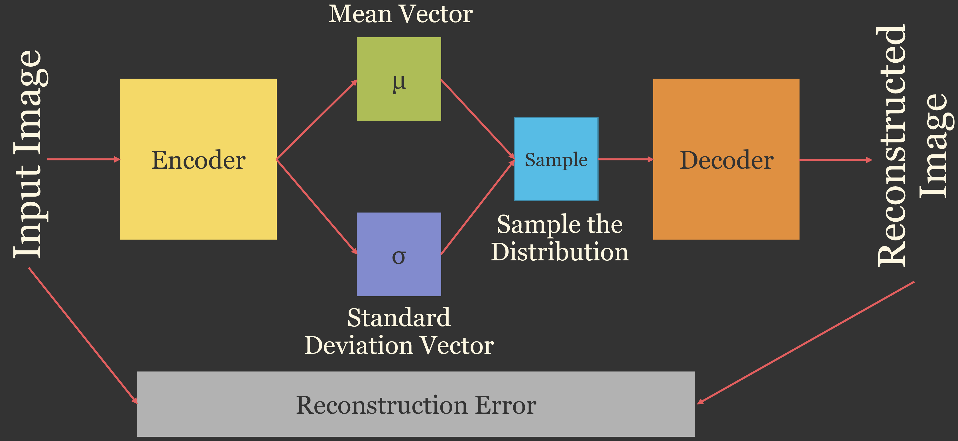
The VAE architecture is conceptualized in Figure 26.1. The encoder compresses the input image to a latent space representation. Unlike a standard autoencoder, which encodes each image as a single point in the latent space, a VAE encodes each image as a probability distribution described by a mean vector (\(\mu\)) and a standard deviation vector (\(\sigma\)). A latent vector is randomly sampled from this distribution and passed to the decoder, which reconstructs the image. The model is trained to minimize the reconstruction error between the input and reconstructed images, along with a term that encourages the latent distributions to be similar to a standard normal distribution. Once trained, images that are poorly reconstructed are potential anomalies.

The example code used here was modified from the following example available on Kaggle: https://www.kaggle.com/code/jaiganesann/vae-implemention-human-rgb-images

26.2 Preparation

As normal, we begin by reading in the required libraries and specifying the device. Since we will use a CNN-based architecture, a CUDA-enabled GPU is necessary to train the model.

import numpy as np
import pandas as pd
import matplotlib
from matplotlib import pyplot as plt

import torch
import torch.nn as nn
import torch.nn.functional as F
from torch.utils.data.dataset import Dataset
from torchvision import transforms
from torch.utils.data import DataLoader

import rasterio as rio

import seaborn as sbn

device = torch.device("cuda:0" if torch.cuda.is_available() else "cpu")
print(device)

cuda:0

I next read in the training and test set CSV files for the EuroSat dataset. We do not need the validation data for this experiment.

Data Location

This chapter uses the multispectral version of the EuroSAT dataset (EuroSATallBands), which is too large to include in the book download and must be downloaded from the source listed in Table 2 (EuroSAT_MS.zip). By default, the code expects the uncompressed EuroSAT_MS folder, which contains one subfolder of images per class, to be saved in the data/files folder (data/files/EuroSAT_MS). If you saved the data elsewhere, set folder below to the folder’s location on your machine.

# Set this to the location of the uncompressed EuroSAT_MS folder on your machine.
folder = "data/files/EuroSAT_MS/"

train = pd.read_csv("data/files/tables/mytrain.csv")
test = pd.read_csv("data/files/tables/mytest.csv")

# The saved partitions (data/files/tables) store paths from the original machine, so point each
# image to its location in the EuroSATallBands folder.
for df in [train, test]:
    df["fullpath"] = folder + df["class"] + "/" + df["file"]

Next, I use Pandas to list the classes differentiated within the EuroSat dataset (“Annual Crop”, “Forest”, “Herbaceous Vegetation”, “Highway”, “Industrial”, “Pasture”, “Permanent Crop”, “Residential”, “River”, and “Sea/Lake”). Using this information, I then filter out all samples not mapped to the “Sea/Lake” class in the training set to a new data frame. I also separate the test data into “Sea/Lake” and “Not Sea/Lake” subsets.

train["class"].unique()

<StringArray>
[          'AnnualCrop',               'Forest', 'HerbaceousVegetation',
              'Highway',           'Industrial',              'Pasture',
        'PermanentCrop',          'Residential',                'River',
              'SeaLake']
Length: 10, dtype: str

train.columns= ['fNm', 'fPth', 'clsNm', 'Clscode']
test.columns= ['fNm', 'fPth', 'clsNm', 'Clscode']

trainNSL = train.query('clsNm != "SeaLake"')
testNSL = test.query('clsNm != "SeaLake"')
testSL = test.query('clsNm =="SeaLake"')

I will need to re-scale the data. In order to accomplish this, I need the band means and standard deviations. So, using the methods already implemented in prior modules I (1) define a function to calculate band means and standard deviations, (2) build a DataSet subclass for the training set, (3) instantiate a DataLoader, and (4) execute the function for the DataLoader.

The DataSet subclass is a bit different from those used in prior modules since I now do not need the class labels or indices: I only need the imagery data. I am also using only a subset of the bands in this experiment: Green, Red, and Near Infrared (NIR).

By printing summary information for a mini-batch of training samples, you can see that the result is a tensor of shape (32, 3, 64, 64). In other words, we are using a mini-batch size of 32 and the images have three channels and 64 rows and columns of pixels. We also confirm that the data are not natively scaled for 0 to 1.

def batch_mean_and_sd(loader, inChn):

    cnt = 0
    fst_moment = torch.empty(inChn)
    snd_moment = torch.empty(inChn)

    for images in loader:
        b, c, h, w = images.shape
        nb_pixels = b * h * w
        sum_ = torch.sum(images, dim=[0, 2, 3])
        sum_of_square = torch.sum(images ** 2,
                                  dim=[0, 2, 3])
        fst_moment = (cnt * fst_moment + sum_) / (cnt + nb_pixels)
        snd_moment = (cnt * snd_moment + sum_of_square) / (cnt + nb_pixels)
        cnt += nb_pixels

    mean, std = fst_moment, torch.sqrt(snd_moment - fst_moment ** 2)
    return mean,std

class EuroSat(Dataset):
  def __init__(self, df):
      super().__init__
      self.df = df

  def __getitem__(self, idx):
      image_name = self.df.iloc[idx, 1]
      source = rio.open(image_name)
      image = source.read()
      source.close()
      image = image.astype('float32')
      image = image[[2,3,7], :, :]
      image = torch.from_numpy(image)
      return image

  def __len__(self):
      return len(self.df)

trainDS = EuroSat(trainNSL)

trainDL = torch.utils.data.DataLoader(trainDS, batch_size=32, shuffle=True, sampler=None,
num_workers=0, pin_memory=False, drop_last=True)

batch = next(iter(trainDL))
images = batch
print(f'Batch Image Shape: {images.shape}')

Batch Image Shape: torch.Size([32, 3, 64, 64])

print(f'Batch Image Data Type: {images.dtype}')

Batch Image Data Type: torch.float32

print(f'Batch Image Band Means: {torch.mean(images, dim=(0,2,3))}')

Batch Image Band Means: tensor([1093.6667, 1033.4270, 2490.7092])

testImg = images[1]
print(f'Image Shape: {testImg.shape}')

Image Shape: torch.Size([3, 64, 64])

print(f'Image Data Type: {testImg.dtype}')

Image Data Type: torch.float32

band_stats = batch_mean_and_sd(trainDL, 3)

band_stats

(tensor([1074.0865, 1000.2383, 2545.3789]), tensor([394.3111, 601.3669, 918.2288]))

I will now re-define the DataSet subclass to apply data transformations. As the VAE is defined, I would like to provide data that have a mean of ~0.5 and a standard deviation of ~0.5 for each channel. In the DataLoader, I apply a normalization using the band means obtained with the custom function. This results in data with a mean of ~0 and a standard deviation of ~1. To adjust the standard deviation to ~0.5, I multiply the re-scaled data by 0.5. I then add 0.5 to adjust the mean from ~0 to ~0.5. I explain why this normalization is required below.

Once the new DataSet subclass is defined, it can be used within a DataLoader. To train the model, I will use a mini-batch size of 32. Each image will have three channels and 64 rows and columns of pixels. By printing a new summary, I can confirm the mini-batch shape. You can also see that the band means and standard deviations are now ~0.5.

transform = transforms.Compose([
    transforms.Normalize(mean=band_stats[0], std=band_stats[1]),
])

class EuroSat(Dataset):
  def __init__(self, df):
      super().__init__
      self.df = df

  def __getitem__(self, idx):
      image_name = self.df.iloc[idx, 1]
      source = rio.open(image_name)
      image = source.read()
      source.close()
      image = image.astype('float32')
      image = image[[2,3,7], :, :]
      image = torch.from_numpy(image)
      image = (transform(image)*0.5)+0.5
      return image

  def __len__(self):
      return len(self.df)

trainDS = EuroSat(trainNSL)

trainDL = torch.utils.data.DataLoader(trainDS, batch_size=32, shuffle=True, sampler=None,
num_workers=0, pin_memory=False, drop_last=True)

batch = next(iter(trainDL))
images = batch
print(f'Batch Image Shape: {images.shape}')

Batch Image Shape: torch.Size([32, 3, 64, 64])

print(f'Batch Image Data Type: {images.dtype}')

Batch Image Data Type: torch.float32

print(f'Batch Image Band Means: {torch.mean(images, dim=(0,2,3))}')

Batch Image Band Means: tensor([0.4841, 0.4888, 0.4672])

testImg = images[1]
print(f'Image Shape: {testImg.shape}')

Image Shape: torch.Size([3, 64, 64])

print(f'Image Data Type: {testImg.dtype}')

Image Data Type: torch.float32

26.3 Define VAE

The next code block defines the VAE. VAEs can be constructed using fully connected-based or CNN-based architectures. Here, I have chosen to use a CNN-based architecture. Both the encoder and decoder have five blocks. The encoder uses strided convolution, as opposed to max pooling, to reduce the size of the array in the spatial dimensions. Through the encoder, the array size is reduced from 64-by-64 to 4-by-4 cells. The number of feature maps increase throughout the encoder. The decoder uses 2D transpose convolution to increase the size of the tensors in the spatial dimensions back to the original size.

Other components of the architecture include fully connected layers for the latent space means and log variances and the re-parameterization required to make the computation differentiable, as required for gradient calculation and backpropagation.

Since the goal is to reconstruct the input data, as opposed to perform classification, the last layer in the decoder applies a sigmoid function and returns a tensor of shape (3, 64, 64). In other words, the architecture returns a three-band image as opposed to logits for predicted classes. Remember that a sigmoid function re-scales data to be between 0 and 1. This is the reason we transformed the input data to have band means of ~0.5 and band standard deviations of ~0.5.

class VAE(nn.Module):
    def __init__(self, latent_dim=64):
        super(VAE, self).__init__()
        self.encoder = nn.Sequential(
            nn.Conv2d(3, 32, kernel_size=3, stride=1, padding=1), # output dimension: 64 X 64 X 32
            nn.ReLU(),
            nn.Conv2d(32, 128, kernel_size=3, stride=1, padding=1), # 64 X 64 X 128
            nn.ReLU(),
            nn.Conv2d(128, 256, kernel_size=4, stride=2, padding=1), # 32 X 32 X 256
            nn.ReLU(),
            nn.Conv2d(256, 512, kernel_size=4, stride=2, padding=1), # 16 X 16 X 512
            nn.ReLU(),
            nn.Conv2d(512, 1024, kernel_size=4, stride=2, padding=1), # 8 X 8 X 1024
            nn.ReLU(),
            nn.Conv2d(1024, 2048, kernel_size=4, stride=2, padding=1), # 4 X 4 X 2048
            nn.ReLU(),
        )

        self.decoder = nn.Sequential(
            nn.ConvTranspose2d(2048, 1024, kernel_size=4, stride=2, padding=1), # Output dimension : 8 X 8 X 1024
            nn.ReLU(),
            nn.ConvTranspose2d(1024, 512, kernel_size=4, stride=2, padding=1), # 16 X 16 X 512
            nn.ReLU(),
            nn.ConvTranspose2d(512, 256, kernel_size=4, stride=2, padding=1), # 32 X 32 X 256
            nn.ReLU(),
            nn.ConvTranspose2d(256, 128, kernel_size=4, stride=2, padding=1), # 64 X 64 X 128
            nn.ReLU(),
            nn.ConvTranspose2d(128, 32, kernel_size=3, stride=1, padding=1), # 64 X 64 X 32
            nn.ReLU(),
            nn.ConvTranspose2d(32, 3, kernel_size=3, stride=1, padding=1),  # 64 X 64 X 3 (Reconstructed image)
            nn.Sigmoid()
        )

        self.fc_mu = nn.Linear(2048*4*4, latent_dim)      # Mean vector from Encoder output
        self.fc_logvar = nn.Linear(2048*4*4, latent_dim)  # Variance Vector from Encoder output

        self.decoder_input = nn.Linear(latent_dim, 2048*4*4) # Latent to decoder output size

    def reparameterize(self, mu, logvar):
        std = torch.exp(0.5 * logvar)
        eps = torch.randn_like(std)
        return mu + eps * std

    def forward(self, x):
        x = self.encoder(x)
        x = x.view(x.size(0), -1)

        mu, logvar = self.fc_mu(x), self.fc_logvar(x)

        z = self.reparameterize(mu, logvar)

        x = self.decoder_input(z)
        x = x.view(x.size(0), 2048, 4, 4)
        x = self.decoder(x)
        return x, mu, logvar

    def decode(self, z):
        x = self.decoder_input(z)
        x = x.view(x.size(0), 2048, 4, 4)
        x = self.decoder(x)
        return x

Once the architecture is defined by subclass nn.Module, I instantiate an instance of the architecture with a latent space dimension size of 256.

vaeModel = VAE(latent_dim = 256).to(device)

26.4 Train VAE

In order to train the VAE, I first instantiate the optimizer: Adam with a learning rate of 1e-3. I also need to define a custom loss function, which is a combination of mean square error (MSE) loss and KL-divergence. MSE loss is used as a measure of reconstruction error while KL-divergence compares the resulting predictions to a Gaussian distribution. The model is penalized for both failing to predict the pixel values accurately and for generating data that do not follow a Gaussian distribution. It is possible to include a weighting term to control the relative impact of the two loss components. I did not do so here.

optimizer = torch.optim.Adam(vaeModel.parameters(), lr=1e-3)

def vaeLoss(x_recon, x, mu, logvar):

    recon_loss = F.mse_loss(x_recon, x, reduction='sum')

    kl_divergence = - 0.5 * torch.sum(1 + logvar - mu.pow(2) - logvar.exp())

    loss = recon_loss + kl_divergence

    return loss, recon_loss, kl_divergence

I now have a DataLoader defined and an instantiated model and optimizer. I have defined a custom loss appropriate for training a VAE. I will now train the model for 30 epochs. The training loop is pretty simple since I am not monitoring a validation datasets. Here are a few key components:

I keep track of all three losses separately
The VAE model returns the prediction for each image within each mini-batch and also the latent space representation
The loss is calculated by comparing the input image and reconstruction

If you choose to execute the training loop, it will take several hours to train the model for 30 epochs. We have provided a trained model if you would like to execute the remaining code without executing the training loop on you machine.

epochs = 30

eNum = []
train_mse = []
train_kld = []
train_loss = []
vaeModel.train()
for epoch in range(epochs):
    batch_loss = 0.0
    batch_mse = 0.0
    batch_kld = 0.0
    for batch in trainDL:
        batch = batch.to(device)  # Move batch to the same device

        optimizer.zero_grad()

        recon_batch, mu, logvar = vaeModel(batch)
        loss, mse, kld = vaeLoss(recon_batch, batch, mu, logvar)

        loss.backward()
        optimizer.step()

        batch_loss += loss.item()
        batch_mse += mse.item()
        batch_kld += kld.item()

    avg_loss = batch_loss / len(trainDL)
    avg_mse = batch_mse / len(trainDL)
    avg_kld = batch_kld / len(trainDL)

    eNum.append(epoch)
    train_mse.append(avg_mse)
    train_kld.append(avg_kld)
    train_loss.append(avg_loss)

    print(f'Epoch [{epoch+1}/{epochs}], Loss: {avg_loss:.4f}, BCE: {avg_mse:.4f}, KLD: {avg_kld:.4f}')

torch.save(vaeModel.state_dict(), "data/output/eurosatVAE.pth")
torch.cuda.empty_cache()

SeNum = pd.Series(eNum, name="epoch")
Strain_mse = pd.Series(train_mse, name="mse")
Strain_kld = pd.Series(train_kld, name="kdl")
Strain_loss = pd.Series(train_loss, name="loss")
resultsDF = pd.concat([SeNum, Strain_mse, Strain_kld, Strain_loss], axis=1)

resultsDF.to_csv("data/output/eurosat_vae_results.csv")

26.5 Explore Model Results

To begin exploring the model, I first plot the loss curve for the combined loss. Generally, it seems that the model has stabilized. Training the model for additional epochs may improve the results, but 30 seems adequate for our experiment.

# Read the training log provided with the text; your own log is saved to data/output/
resultsDF = pd.read_csv("data/models/eurosat_vae_results.csv")

plt.rcParams['figure.figsize'] = [10, 10]
firstPlot = resultsDF.plot(x='epoch', y="loss")
plt.show()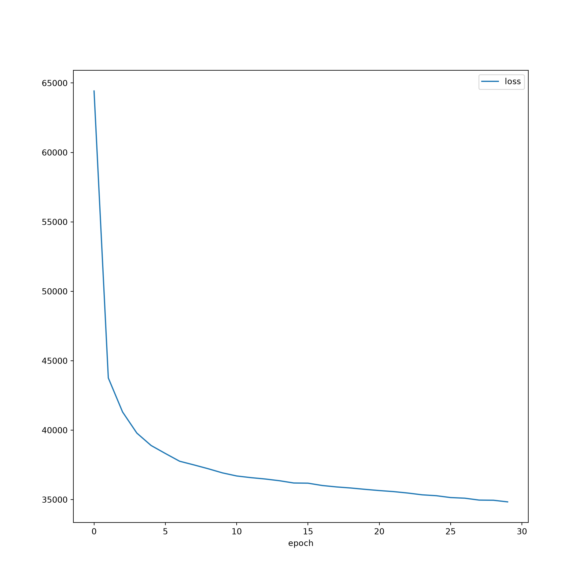

Next, I instantiate a new model and load the saved parameters from disk. Again, the trained model has been provided.

vaeModel = VAE(latent_dim = 256).to(device)
best_weights = torch.load("data/models/eurosatVAE.pth")
vaeModel.load_state_dict(best_weights)

<All keys matched successfully>

I generate DataSets and DataLoaders for the two test set subsets: “Not Sea/Lake” and “Sea/Lake”. Remember that the model was trained using only “Not Sea/Lake” samples. As a result, we would expect it to do a poorer job reconstructing “Sea/Lake” samples in comparison to those from other classes. I will test this now. In my new DataLoader, I am going to predict each image separately by using a mini-batch size of 1. Also, I am now interested in the reconstruction error specifically; as a result, I redefine a loss function that only considers the MSE loss.

testDSNSL = EuroSat(testNSL)
testDSSL = EuroSat(testSL)

testDLNSL = torch.utils.data.DataLoader(testDSNSL, batch_size=1, shuffle=False, sampler=None,
num_workers=0, pin_memory=False, drop_last=True)

testDLSL = torch.utils.data.DataLoader(testDSSL, batch_size=1, shuffle=False, sampler=None,
num_workers=0, pin_memory=False, drop_last=True)

def reconstruction_loss(x_recon, x):

    recon_loss = F.mse_loss(x_recon, x, reduction='sum')

    return recon_loss

I now execute a validation loop for each test set subset. The resulting reconstruction losses for each image are saved to disk as a CSV file.

all_lossesSL = []
vaeModel.eval()
for batch in testDLSL:
  batch = batch.to(device)
  recon_batch, mu, logvar = vaeModel(batch)
  loss = reconstruction_loss(recon_batch, batch)

  current_loss = loss.item()
  all_lossesSL.append(current_loss)
torch.cuda.empty_cache()

slLosses = pd.Series(all_lossesSL, name="Reconstruction_Loss")
slDF = pd.concat([slLosses], axis=1)
slDF["Set"] = "Sea/Lake"
slDF.to_csv("data/output/slPredictions.csv")

all_lossesNSL = []
vaeModel.eval()
for batch in testDLNSL:
  batch = batch.to(device)
  recon_batch, mu, logvar = vaeModel(batch)
  loss = reconstruction_loss(recon_batch, batch)

  current_loss = loss.item()
  all_lossesNSL.append(current_loss)
torch.cuda.empty_cache()

nslLosses = pd.Series(all_lossesNSL, name="Reconstruction_Loss")
nslDF = pd.concat([nslLosses], axis=1)
nslDF["Set"] = "Other"
nslDF.to_csv("data/output/nslPredictions.csv")

I next read in the saved reconstruction loss CSV files from disk, extract a subsample to speed up the computation and balance the number of samples in each class, and build a new data frame containing the balanced subset. Seaborn is used to generate a grouped kernel density plot.

Generally, the results suggest that the model is doing a better job predicting “Not Sea/Lake” samples in comparison to “Sea/Lake” samples; however, there is some overlap in the distributions. In order to use the trained model as an anomaly detector, I could set a reconstruction error threshold to use to flag samples as anomalies. I could then pass new data to the model and label any sample with a reconstruction loss larger than the defined threshold as an anomaly. In order to quantify the accuracy of the detector, I could pass labeled data through the model, label the results as anomalies or not using the defined threshold, and use the actual and predicted labels to count true positive, true negative, false positive, and false negative results and generate assessment metrics.

# Read the predictions provided with the text; your own predictions are saved to data/output/
slResults = pd.read_csv("data/models/slPredictions.csv")
nslResults = pd.read_csv("data/models/nslPredictions.csv")

slResultsSub = slResults.sample(n=400)
nslResultsSub = nslResults.sample(n=400)
allResults = pd.concat([slResultsSub, nslResultsSub], axis=0)

sbn.kdeplot(data=allResults, x="Reconstruction_Loss", hue="Set", alpha=0.4)
plt.show()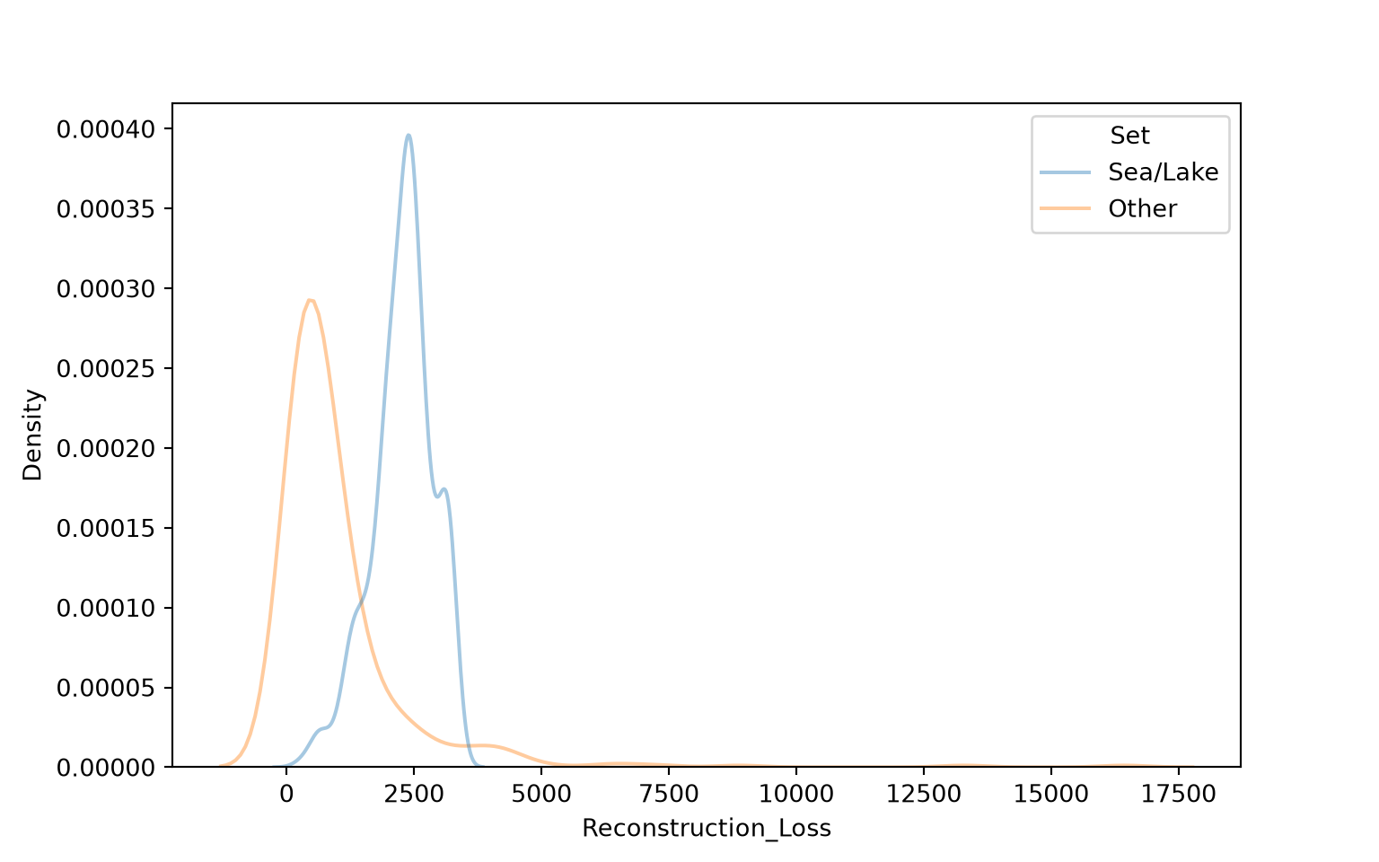

As a final check of the model, I predict a “Not Sea/Lake” sample and a “Sea/Lake” sample from the test sets then print the original image and reconstruction using matplotlib. You may notice that the reconstructions are a bit blurry. This is a common issue with VAEs when the data are used to generate synthetic data or for compression. In our anomaly detection use case, this is less of a concern.

Since the data were normalized using the band means and standard deviations of the “Not Sea/Lake” training samples, the pixel values are not guaranteed to fall within the 0 to 1 range expected by matplotlib. Water bodies have low reflectance in the Green, Red, and NIR bands, so the normalized “Sea/Lake” values are generally negative and would display as black. To visualize the chips, I define a function that applies a 2% to 98% percentile stretch to each band.

def stretch(img, lo=2, hi=98):
    p_lo, p_hi = np.percentile(img, [lo, hi], axis=(0, 1))
    return np.clip((img - p_lo) / (p_hi - p_lo + 1e-8), 0, 1)

batch = next(iter(testDLNSL))
imgIn = batch.to(device)
recon_img, mu, logvar = vaeModel(imgIn)
imgOrig = (imgIn.squeeze().permute(1, 2, 0).detach().cpu().numpy())
imgPred = (recon_img.squeeze().permute(1, 2, 0).detach().cpu().numpy())

fig, axs = plt.subplots(1, 2, figsize=(10, 5))

axs[0].imshow(stretch(imgOrig))
axs[0].set_title('Original Chip')
axs[0].axis('off')

axs[1].imshow(stretch(imgPred))
axs[1].set_title('Reconstructed Chip')
axs[1].axis('off')

plt.show()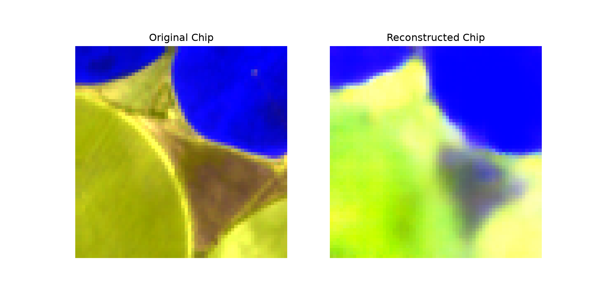

batch = next(iter(testDLSL))
imgIn = batch.to(device)
recon_img, mu, logvar = vaeModel(imgIn)
imgOrig = (imgIn.squeeze().permute(1, 2, 0).detach().cpu().numpy())
imgPred = (recon_img.squeeze().permute(1, 2, 0).detach().cpu().numpy())

fig, axs = plt.subplots(1, 2, figsize=(10, 5))

axs[0].imshow(stretch(imgOrig))
axs[0].set_title('Original Chip')
axs[0].axis('off')

axs[1].imshow(stretch(imgPred))
axs[1].set_title('Reconstructed Chip')
axs[1].axis('off')

plt.show()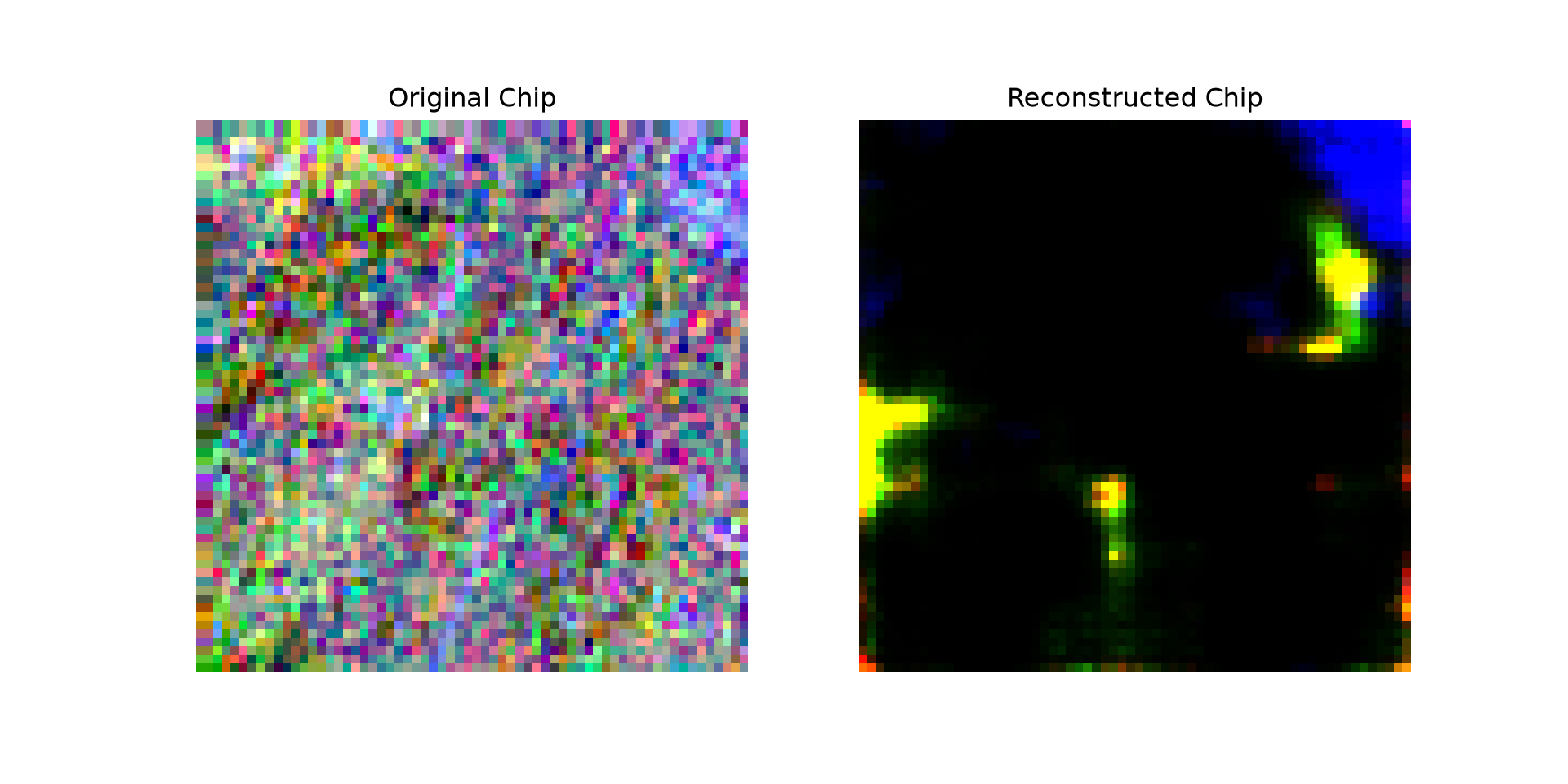

26.6 Concluding Remarks

The primary goal of this module was to demonstrate a different use case of deep learning in the geospatial sciences: variational autoencoders for anomaly detection. One of the strengths of deep learning architectures is their flexibility and application to a variety of use cases, not just predictive modeling or classification/regression tasks.

26.7 Questions

Explain how a variational autoencoder (VAE) can be used to detect anomalies.
Why was the VAE trained using only samples that were not from the “Sea/Lake” class?
Explain the two components of the loss function used to train the VAE. What does each component penalize?
What is the reparameterization trick, and why is it necessary to train a VAE?
Why were the input data normalized to have band means of ~0.5 and band standard deviations of ~0.5? How does this relate to the activation function applied at the end of the decoder?
How did the encoder in this chapter’s VAE reduce the size of the tensors in the spatial dimensions? How does this differ from the CNN architectures explored in earlier chapters?
Explain how a reconstruction error threshold could be selected and how the accuracy of the resulting anomaly detector could be assessed.
Why are the reconstructions generated by a VAE often blurry? Why is this less of a concern for anomaly detection than for generating synthetic data?

26.8 Exercises

Exercise 26.1: Detect Surface Mining using a VAE

Introduction

The goal of this exercise is to build an anomaly detection algorithm using a variational autoencoder (VAE) that detects sections of topographic maps that include surface mine disturbance as anomalies.

Deliverables

A Quarto (.qmd) file containing all required code and answers to the questions and discussion prompts, and the HTML webpage rendered from it

Data

This exercise uses the topoDLMini dataset, a subset of the topoDL dataset, which was used in Chapter 21. It is provided as a separate download (topoDLMini.zip) in the download menu in the sidebar. By default, the chapter code expects the uncompressed topoDLMini folder to be saved in the data/files folder (data/files/topoDLMini).

Background Questions

Question 1: Explain the difference between an autoencoder and a variational autoencoder.

Question 2: Explain the concept of a latent space.

Question 3: Explain the reparameterization trick required to implement VAEs and why it is necessary.

Question 4: Explain the loss function for a VAE. What is the purpose of the reconstruction loss and the KL-divergence loss?

Tasks

Edit the anomaly detection example from this chapter to detect chips in the topoDLMini dataset that include mine disturbance as anomalies. This will involve training a model using only the background chips. The code should include the following components.

Read in the trainDF.csv and testDF.csv files from the topoDLMini folder as Pandas DataFrames. You will not need the validation set data.
Subset out only the “background” training samples.
Split the test set samples into separate “background” and “positive” sets.
Use the DataFrames to create a DataSet subclass that reads in the topographic map images and their associated label: “positive” or “background”. You will not need the masks. Make sure the topographic map chips are rescaled from 0 to 1 and converted to a 32-bit float data type. The “background” and “positive” cases should be assigned unique numeric codes with a long integer data type.
Instantiate DataSets and DataLoaders for the “background”-only training set, “background”-only test set, and “positive”-only test set.
Define a VAE architecture. You can use the architecture defined in this chapter.
Define a VAE loss. You can implement the loss from this chapter, which sums the MSE and KL-divergence losses.
Instantiate the model.
Train the model for at least 30 epochs.
Use the trained model to predict the “background”-only and “positive”-only test sets separately. Create a grouped kernel density plot showing the distribution of the reconstruction loss for the “background”-only and “positive”-only test sets (like the one in this chapter).
Using the graph, discuss the results. Could the model be used to detect topographic map chips that include surface mining? If so, what reconstruction loss threshold would you suggest using?