import numpy as np
import pandas as pd
import matplotlib
from matplotlib import pyplot as plt
import seaborn as sns

import os
from sklearn import preprocessing
from sklearn.metrics import confusion_matrix
from sklearn.metrics import classification_report

import torch
import torch.nn as nn
from torch.utils.data.dataset import Dataset
from torch.utils.data import DataLoader

import rasterio as rio

import torchmetrics as tm

from torchinfo import summary

import torchvision
import torchvision.transforms as transforms13 Transfer Learning and CNNs
13.1 Introduction
In this last chapter focused on CNNs for scene classification or scene labeling, we will experiment with transfer learning for classifying the EuroSatAllBands dataset. Specifically, we will use a modified ResNet-34 architecture initialized using pre-trained weights from ImageNet. The majority of the code that you will see in this module is not new, so I will keep my explanations brief. As this module demonstrates, once you have learned the key components of implementing deep learning with PyTorch, it is possible to use your knowledge and adapt your or another analyst’s code to a new purpose or problem.
13.2 Preparation
Here is a quick review of the steps required to prepare the EuroSatAllBands data for input into a CNN architecture designed for scene labeling.
- Import the required libraries. This includes NumPy, Pandas, matplotlib, Seaborn, os, torch, torch.nn, torch.utils.data.dataset, torch.utils.data, Rasterio, torchmetrics, torchinfo, torchvision, and torchvision.transforms. I also import some specific assessment functions from scikit-learn.
- Set the device variable to the GPU if one is available.
- Set the folder path to the data to the folder variable.
- Read in the data tables of image chips using Pandas. Here, I am also augmenting the file path since I am working on a different computer with a different directory structure.
- Define a DataSet subclass to obtain the band statistics.
- Instantiate a DataSet for the training set.
- Define a DataLoader for the DataSet.
- Define a function to calculate the pixel-level band means and standard deviations.
- Calculate the band means and standard deviations.
- Define a DataSet subclass for use in the training and validation process that accepts a DataFrame containing the information for each image chip, the band means and standard deviations, and transforms.
- Further prepare the band means and standard deviations to create tensors with the same shape as the input image chips (10, 64, 64).
- Define transforms for the training data. Here, I am using random horizontal and vertical flips.
- Instantiate an instance of the DataSet class for the training data that uses the defined transforms and an instance of the validation data that does not apply the transforms.
- Define the DataLoader for the training and validation data. I am using a mini-batch size of 32 here as this worked on my hardware. You may need to change this depending on your system and GPU specifications.
- Perform checks to make sure the mini-batch shapes and data types are correct. Also, check a single image chip.
- Define a function to display a mini-batch of images and their associated labels.
- Visualize a mini-batch of images and their associated labels.
device = torch.device("cuda:0" if torch.cuda.is_available() else "cpu")
print(device)
cuda:0
ImportantData Location
This chapter uses the multispectral version of the EuroSAT dataset (EuroSATallBands), which is too large to include in the book download and must be downloaded from the source listed in Table 2 (EuroSAT_MS.zip). By default, the code expects the uncompressed EuroSAT_MS folder, which contains one subfolder of images per class, to be saved in the data/files folder (data/files/EuroSAT_MS). If you saved the data elsewhere, set folder below to the folder’s location on your machine.
# Set this to the location of the uncompressed EuroSAT_MS folder on your machine.
folder = "data/files/EuroSAT_MS/"
train = pd.read_csv("data/files/tables/mytrain.csv")
test = pd.read_csv("data/files/tables/mytest.csv")
val = pd.read_csv("data/files/tables/myval.csv")
# The saved partitions (data/files/tables) store paths from the original machine, so point each
# image to its location in the EuroSATallBands folder.
for df in [train, test, val]:
df["fullpath"] = folder + df["class"] + "/" + df["file"]class EuroSat(Dataset):
def __init__(self, df):
super().__init__
self.df = df
def __getitem__(self, idx):
image_name = self.df.iloc[idx, 1]
label = self.df.iloc[idx, 3]
label = np.array(label)
source = rio.open(image_name)
image = source.read()
source.close()
image = image.astype('float32')
image = image[[1,2,3,4,5,6,7,8,11,12], :, :]
image = torch.from_numpy(image)
label = torch.from_numpy(label)
label = label.long()
return image, label
def __len__(self):
return len(self.df)trainDS = EuroSat(train)
print(len(trainDS))16200trainDL = torch.utils.data.DataLoader(trainDS, batch_size=32, shuffle=True, sampler=None,
num_workers=0, pin_memory=False, drop_last=False)#https://www.binarystudy.com/2021/04/how-to-calculate-mean-standard-deviation-images-pytorch.html
def batch_mean_and_sd(loader, inChn):
cnt = 0
sums = torch.zeros(inChn, dtype=torch.float64)
sq_sums = torch.zeros(inChn, dtype=torch.float64)
for images, _ in loader:
images = images.double()
b, c, h, w = images.shape
cnt += b * h * w
sums += images.sum(dim=[0, 2, 3])
sq_sums += (images ** 2).sum(dim=[0, 2, 3])
mean = sums / cnt
std = torch.sqrt(sq_sums / cnt - mean ** 2)
return mean.float(), std.float()band_stats = batch_mean_and_sd(trainDL, 10)class EuroSat(Dataset):
def __init__(self, df, mnImg, sdImg, transform):
self.df = df
self.mnImg = mnImg
self.sdImg = sdImg
self.transform = transform
def __getitem__(self, idx):
image_name = self.df.iloc[idx, 1]
label = self.df.iloc[idx, 3]
label = np.array(label)
source = rio.open(image_name)
image = source.read()
source.close()
image = image[[1,2,3,4,5,6,7,8,11,12], :, :]
image = np.subtract(image, self.mnImg)
image = np.divide(image, self.sdImg)
image = image.astype('float32')
image = torch.from_numpy(image)
label = torch.from_numpy(label)
label = label.long()
if self.transform is not None:
image = self.transform(image)
return image, label
def __len__(self):
return len(self.df)bndMns = np.array(band_stats[0].tolist())
bndSDs = np.array(band_stats[1].tolist())mnImg = np.repeat(bndMns[0], 64*64).reshape((64,64,1))
for b in range(1,len(bndMns)):
mnImg2 = np.repeat(bndMns[b], 64*64).reshape((64,64,1))
mnImg = np.dstack([mnImg, mnImg2])
mnImg = np.transpose(mnImg, (2,0,1))
sdImg = np.repeat(bndSDs[0], 64*64).reshape((64,64,1))
for b in range(1,len(bndSDs)):
sdImg2 = np.repeat(bndSDs[b], 64*64).reshape((64,64,1))
sdImg = np.dstack([sdImg, sdImg2])
sdImg = np.transpose(sdImg, (2,0,1))
print(mnImg.shape)(10, 64, 64)print(sdImg.shape)(10, 64, 64)myTransforms = transforms.Compose(
[transforms.RandomHorizontalFlip(p=0.3),
transforms.RandomVerticalFlip(p=0.3),]
)trainDS = EuroSat(train, mnImg, sdImg, transform=myTransforms)
valDS = EuroSat(val, mnImg, sdImg, transform=None)trainDL = torch.utils.data.DataLoader(trainDS, batch_size=32, shuffle=True, sampler=None,
num_workers=0, pin_memory=False, drop_last=True)
valDL = torch.utils.data.DataLoader(valDS, batch_size=32, shuffle=False, sampler=None,
num_workers=0, pin_memory=False, drop_last=True)batch = next(iter(trainDL))
images, labels = batch
print(f'Batch Image Shape: {images.shape}, Batch Label Shape: {labels.shape}')Batch Image Shape: torch.Size([32, 10, 64, 64]), Batch Label Shape: torch.Size([32])print(f'Batch Image Data Type: {images.dtype}, Batch Label Data Type: {labels.dtype}')Batch Image Data Type: torch.float32, Batch Label Data Type: torch.int64print(f'Batch Image Band Means: {torch.mean(images, dim=(0,2,3))}')Batch Image Band Means: tensor([-0.0554, -0.0835, -0.0323, -0.0527, 0.0024, 0.0186, 0.0108, -0.0597,
-0.0441, 0.0240])print(f'Batch Label Minimum: {torch.min(labels, dim=0)}, Batch Label Maximum: {torch.max(labels, dim=0)}')Batch Label Minimum: torch.return_types.min(
values=tensor(0),
indices=tensor(0)), Batch Label Maximum: torch.return_types.max(
values=tensor(9),
indices=tensor(6))testImg = images[1]
testMsk = labels[1]
print(f'Image Shape: {testImg.shape}, Label Shape: {testMsk.shape}')Image Shape: torch.Size([10, 64, 64]), Label Shape: torch.Size([])print(f'Image Data Type: {testImg.dtype}, Label Data Type: {testMsk.dtype}')Image Data Type: torch.float32, Label Data Type: torch.int64def img_display(img, mnImg, sdImg):
img = np.multiply(img, sdImg)
img = np.add(img, mnImg)
image_vis = img[[2,1,0],:,:]
image_vis = image_vis.permute(1,2,0)
image_vis = (image_vis.numpy()/4000)*255
image_vis = image_vis.astype('uint8')
return image_vis
batch = next(iter(trainDL))
images, labels = batch
cover_types = {0: 'Annual Crop',
1: 'Forest',
2: 'Herb Veg',
3: 'Highway',
4: 'Industrial',
5: 'Pasture',
6: 'Perm Crop',
7: 'Residential',
8: 'River',
9: 'SeaLake'}fig, axis = plt.subplots(4, 8, figsize=(15, 10))
for i, ax in enumerate(axis.flat):
with torch.no_grad():
image, label = images[i], labels[i]
ax.imshow(img_display(image, mnImg, sdImg)) # add image
ax.set(title = f"{cover_types[label.item()]}") # add label
ax.axis('off')
plt.show()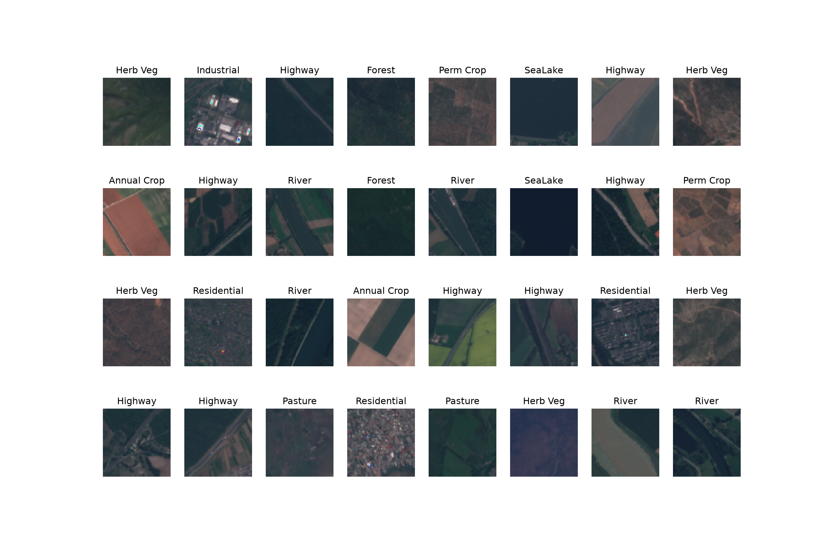
13.3 Instantiate Pre-trained Model
The next set of code comes from the prior modules associated with CNN architectures. I first define a function to freeze weights. I next define a function to instantiate a ResNet model. This function allows the user to select a ResNet architecture (“18”, “34”, “50”, “101”, or “152”), the number of input channels, the number of classes being differentiated, whether or not to freeze the parameters/weights associated with the convolutional component of the model, and whether or not to use the pre-trained weights from ImageNet.
I instantiate a model instance using the defined function. I will use a ResNet-34 architecture that expects 10 input channels, differentiates 10 classes, does not have any weights frozen (i.e., all weights will be able to be updated), and that uses pre-trained weights from ImageNet. So, this model will be initialized using the ImageNet weights, other than the first convolutional layer and batch normalization layer and the fully connected layer at the end of the model. However, all weights will be trainable. This is because this problem is very different from the ImageNet use case. Thus, it is expected that the parameters/weights learned from ImageNet within the convolutional component of the model will need to be updated to allow the model to learn spatial patterns useful for this specific problem.
Once the model is initialized, I summarize it using torchinfo and the mini-batch size and tensor shape of the EuroSatAllBands dataset: (32,10,64,64). This model has > 21 million trainable parameters. Since no parameters/weights were frozen, there are no non-trainable parameters.
#https://pytorch.org/tutorials/beginner/finetuning_torchvision_models_tutorial.html
def set_parameter_requires_grad(model, freeze=True):
    if freeze == True:
        for param in model.parameters():
            param.requires_grad = False
# https://stackoverflow.com/questions/62629114/how-to-modify-resnet-50-with-4-channels-as-input-using-pre-trained-weights-in-py
# https://discuss.pytorch.org/t/transfer-learning-usage-with-different-input-size/20744
def initialize_model(resNet, nChn, nCls, freeze=True, pretrained=True):
weights = "DEFAULT" if pretrained else None
if resNet == "18":
model = torchvision.models.resnet18(weights=weights)
elif resNet == "34":
model = torchvision.models.resnet34(weights=weights)
elif resNet == "50":
model = torchvision.models.resnet50(weights=weights)
elif resNet == "101":
model = torchvision.models.resnet101(weights=weights)
elif resNet == "152":
model = torchvision.models.resnet152(weights=weights)
else:
model = torchvision.models.resnet34(weights=weights)
if pretrained == True:
set_parameter_requires_grad(model, freeze)
# Replace the head so the model outputs nCls logits (always, even without pre-trained weights)
num_ftrs = model.fc.in_features
model.fc = nn.Linear(num_ftrs, nCls)
if nChn != 3:
model.conv1 = nn.Conv2d(nChn, 64, kernel_size=7, stride=2, padding=3, bias=False)
model.bn1 = nn.BatchNorm2d(64)
return modelmodel = initialize_model(resNet="34", nChn=10, nCls=10, freeze=False, pretrained=True).to(device)summary(model, (32, 10, 64, 64))==========================================================================================
Layer (type:depth-idx) Output Shape Param #
==========================================================================================
ResNet [32, 10] --
├─Conv2d: 1-1 [32, 64, 32, 32] 31,360
├─BatchNorm2d: 1-2 [32, 64, 32, 32] 128
├─ReLU: 1-3 [32, 64, 32, 32] --
├─MaxPool2d: 1-4 [32, 64, 16, 16] --
├─Sequential: 1-5 [32, 64, 16, 16] --
│ └─BasicBlock: 2-1 [32, 64, 16, 16] --
│ │ └─Conv2d: 3-1 [32, 64, 16, 16] 36,864
│ │ └─BatchNorm2d: 3-2 [32, 64, 16, 16] 128
│ │ └─ReLU: 3-3 [32, 64, 16, 16] --
│ │ └─Conv2d: 3-4 [32, 64, 16, 16] 36,864
│ │ └─BatchNorm2d: 3-5 [32, 64, 16, 16] 128
│ │ └─ReLU: 3-6 [32, 64, 16, 16] --
│ └─BasicBlock: 2-2 [32, 64, 16, 16] --
│ │ └─Conv2d: 3-7 [32, 64, 16, 16] 36,864
│ │ └─BatchNorm2d: 3-8 [32, 64, 16, 16] 128
│ │ └─ReLU: 3-9 [32, 64, 16, 16] --
│ │ └─Conv2d: 3-10 [32, 64, 16, 16] 36,864
│ │ └─BatchNorm2d: 3-11 [32, 64, 16, 16] 128
│ │ └─ReLU: 3-12 [32, 64, 16, 16] --
│ └─BasicBlock: 2-3 [32, 64, 16, 16] --
│ │ └─Conv2d: 3-13 [32, 64, 16, 16] 36,864
│ │ └─BatchNorm2d: 3-14 [32, 64, 16, 16] 128
│ │ └─ReLU: 3-15 [32, 64, 16, 16] --
│ │ └─Conv2d: 3-16 [32, 64, 16, 16] 36,864
│ │ └─BatchNorm2d: 3-17 [32, 64, 16, 16] 128
│ │ └─ReLU: 3-18 [32, 64, 16, 16] --
├─Sequential: 1-6 [32, 128, 8, 8] --
│ └─BasicBlock: 2-4 [32, 128, 8, 8] --
│ │ └─Conv2d: 3-19 [32, 128, 8, 8] 73,728
│ │ └─BatchNorm2d: 3-20 [32, 128, 8, 8] 256
│ │ └─ReLU: 3-21 [32, 128, 8, 8] --
│ │ └─Conv2d: 3-22 [32, 128, 8, 8] 147,456
│ │ └─BatchNorm2d: 3-23 [32, 128, 8, 8] 256
│ │ └─Sequential: 3-24 [32, 128, 8, 8] 8,448
│ │ └─ReLU: 3-25 [32, 128, 8, 8] --
│ └─BasicBlock: 2-5 [32, 128, 8, 8] --
│ │ └─Conv2d: 3-26 [32, 128, 8, 8] 147,456
│ │ └─BatchNorm2d: 3-27 [32, 128, 8, 8] 256
│ │ └─ReLU: 3-28 [32, 128, 8, 8] --
│ │ └─Conv2d: 3-29 [32, 128, 8, 8] 147,456
│ │ └─BatchNorm2d: 3-30 [32, 128, 8, 8] 256
│ │ └─ReLU: 3-31 [32, 128, 8, 8] --
│ └─BasicBlock: 2-6 [32, 128, 8, 8] --
│ │ └─Conv2d: 3-32 [32, 128, 8, 8] 147,456
│ │ └─BatchNorm2d: 3-33 [32, 128, 8, 8] 256
│ │ └─ReLU: 3-34 [32, 128, 8, 8] --
│ │ └─Conv2d: 3-35 [32, 128, 8, 8] 147,456
│ │ └─BatchNorm2d: 3-36 [32, 128, 8, 8] 256
│ │ └─ReLU: 3-37 [32, 128, 8, 8] --
│ └─BasicBlock: 2-7 [32, 128, 8, 8] --
│ │ └─Conv2d: 3-38 [32, 128, 8, 8] 147,456
│ │ └─BatchNorm2d: 3-39 [32, 128, 8, 8] 256
│ │ └─ReLU: 3-40 [32, 128, 8, 8] --
│ │ └─Conv2d: 3-41 [32, 128, 8, 8] 147,456
│ │ └─BatchNorm2d: 3-42 [32, 128, 8, 8] 256
│ │ └─ReLU: 3-43 [32, 128, 8, 8] --
├─Sequential: 1-7 [32, 256, 4, 4] --
│ └─BasicBlock: 2-8 [32, 256, 4, 4] --
│ │ └─Conv2d: 3-44 [32, 256, 4, 4] 294,912
│ │ └─BatchNorm2d: 3-45 [32, 256, 4, 4] 512
│ │ └─ReLU: 3-46 [32, 256, 4, 4] --
│ │ └─Conv2d: 3-47 [32, 256, 4, 4] 589,824
│ │ └─BatchNorm2d: 3-48 [32, 256, 4, 4] 512
│ │ └─Sequential: 3-49 [32, 256, 4, 4] 33,280
│ │ └─ReLU: 3-50 [32, 256, 4, 4] --
│ └─BasicBlock: 2-9 [32, 256, 4, 4] --
│ │ └─Conv2d: 3-51 [32, 256, 4, 4] 589,824
│ │ └─BatchNorm2d: 3-52 [32, 256, 4, 4] 512
│ │ └─ReLU: 3-53 [32, 256, 4, 4] --
│ │ └─Conv2d: 3-54 [32, 256, 4, 4] 589,824
│ │ └─BatchNorm2d: 3-55 [32, 256, 4, 4] 512
│ │ └─ReLU: 3-56 [32, 256, 4, 4] --
│ └─BasicBlock: 2-10 [32, 256, 4, 4] --
│ │ └─Conv2d: 3-57 [32, 256, 4, 4] 589,824
│ │ └─BatchNorm2d: 3-58 [32, 256, 4, 4] 512
│ │ └─ReLU: 3-59 [32, 256, 4, 4] --
│ │ └─Conv2d: 3-60 [32, 256, 4, 4] 589,824
│ │ └─BatchNorm2d: 3-61 [32, 256, 4, 4] 512
│ │ └─ReLU: 3-62 [32, 256, 4, 4] --
│ └─BasicBlock: 2-11 [32, 256, 4, 4] --
│ │ └─Conv2d: 3-63 [32, 256, 4, 4] 589,824
│ │ └─BatchNorm2d: 3-64 [32, 256, 4, 4] 512
│ │ └─ReLU: 3-65 [32, 256, 4, 4] --
│ │ └─Conv2d: 3-66 [32, 256, 4, 4] 589,824
│ │ └─BatchNorm2d: 3-67 [32, 256, 4, 4] 512
│ │ └─ReLU: 3-68 [32, 256, 4, 4] --
│ └─BasicBlock: 2-12 [32, 256, 4, 4] --
│ │ └─Conv2d: 3-69 [32, 256, 4, 4] 589,824
│ │ └─BatchNorm2d: 3-70 [32, 256, 4, 4] 512
│ │ └─ReLU: 3-71 [32, 256, 4, 4] --
│ │ └─Conv2d: 3-72 [32, 256, 4, 4] 589,824
│ │ └─BatchNorm2d: 3-73 [32, 256, 4, 4] 512
│ │ └─ReLU: 3-74 [32, 256, 4, 4] --
│ └─BasicBlock: 2-13 [32, 256, 4, 4] --
│ │ └─Conv2d: 3-75 [32, 256, 4, 4] 589,824
│ │ └─BatchNorm2d: 3-76 [32, 256, 4, 4] 512
│ │ └─ReLU: 3-77 [32, 256, 4, 4] --
│ │ └─Conv2d: 3-78 [32, 256, 4, 4] 589,824
│ │ └─BatchNorm2d: 3-79 [32, 256, 4, 4] 512
│ │ └─ReLU: 3-80 [32, 256, 4, 4] --
├─Sequential: 1-8 [32, 512, 2, 2] --
│ └─BasicBlock: 2-14 [32, 512, 2, 2] --
│ │ └─Conv2d: 3-81 [32, 512, 2, 2] 1,179,648
│ │ └─BatchNorm2d: 3-82 [32, 512, 2, 2] 1,024
│ │ └─ReLU: 3-83 [32, 512, 2, 2] --
│ │ └─Conv2d: 3-84 [32, 512, 2, 2] 2,359,296
│ │ └─BatchNorm2d: 3-85 [32, 512, 2, 2] 1,024
│ │ └─Sequential: 3-86 [32, 512, 2, 2] 132,096
│ │ └─ReLU: 3-87 [32, 512, 2, 2] --
│ └─BasicBlock: 2-15 [32, 512, 2, 2] --
│ │ └─Conv2d: 3-88 [32, 512, 2, 2] 2,359,296
│ │ └─BatchNorm2d: 3-89 [32, 512, 2, 2] 1,024
│ │ └─ReLU: 3-90 [32, 512, 2, 2] --
│ │ └─Conv2d: 3-91 [32, 512, 2, 2] 2,359,296
│ │ └─BatchNorm2d: 3-92 [32, 512, 2, 2] 1,024
│ │ └─ReLU: 3-93 [32, 512, 2, 2] --
│ └─BasicBlock: 2-16 [32, 512, 2, 2] --
│ │ └─Conv2d: 3-94 [32, 512, 2, 2] 2,359,296
│ │ └─BatchNorm2d: 3-95 [32, 512, 2, 2] 1,024
│ │ └─ReLU: 3-96 [32, 512, 2, 2] --
│ │ └─Conv2d: 3-97 [32, 512, 2, 2] 2,359,296
│ │ └─BatchNorm2d: 3-98 [32, 512, 2, 2] 1,024
│ │ └─ReLU: 3-99 [32, 512, 2, 2] --
├─AdaptiveAvgPool2d: 1-9 [32, 512, 1, 1] --
├─Linear: 1-10 [32, 10] 5,130
==========================================================================================
Total params: 21,311,754
Trainable params: 21,311,754
Non-trainable params: 0
Total mult-adds (Units.GIGABYTES): 10.29
==========================================================================================
Input size (MB): 5.24
Forward/backward pass size (MB): 156.24
Params size (MB): 85.25
Estimated Total Size (MB): 246.73
==========================================================================================13.4 Train with Lightning
I am now ready to train the model using PyTorch Lightning. The simplest approach is to use the LitClassifier LightningModule defined in Chapter 10, which applies a single learning rate to all of the parameters in the model. This is how the provided model was trained: all parameters were updated using the AdamW optimizer with its default learning rate of 0.001 for 50 epochs, saving the model that provided the largest class-aggregated F1-score for the validation data.
import lightning as L
from lightning.pytorch.callbacks import ModelCheckpoint, LearningRateMonitor, BaseFinetuning
from lightning.pytorch.loggers import CSVLogger

class LitClassifier(L.LightningModule):
    def __init__(self, model, nCls, lr=1e-3):
        super().__init__()
        self.save_hyperparameters(ignore=["model"])
        self.model = model
        self.criterion = nn.CrossEntropyLoss()
        self.lr = lr
        metrics = tm.MetricCollection({
            "acc": tm.Accuracy(task="multiclass", num_classes=nCls),
            "f1": tm.F1Score(task="multiclass", num_classes=nCls, average="macro"),
            "kappa": tm.CohenKappa(task="multiclass", num_classes=nCls),
        })
        self.train_metrics = metrics.clone(prefix="train_")
        self.val_metrics = metrics.clone(prefix="val_")
        self.test_metrics = metrics.clone(prefix="test_")

    def forward(self, x):
        return self.model(x)

    def _shared_step(self, batch, metrics, stage):
        x, y = batch
        logits = self(x)
        loss = self.criterion(logits, y)
        metrics.update(logits, y)
        self.log(f"{stage}_loss", loss, on_step=False, on_epoch=True, prog_bar=True)
        self.log_dict(metrics, on_step=False, on_epoch=True, prog_bar=(stage == "val"))
        return loss

    def training_step(self, batch, batch_idx):
        return self._shared_step(batch, self.train_metrics, "train")

    def validation_step(self, batch, batch_idx):
        self._shared_step(batch, self.val_metrics, "val")

    def test_step(self, batch, batch_idx):
        self._shared_step(batch, self.test_metrics, "test")

    def predict_step(self, batch, batch_idx):
        x = batch[0] if isinstance(batch, (list, tuple)) else batch
        return torch.softmax(self(x), dim=1)

    def configure_optimizers(self):
        return torch.optim.AdamW(self.parameters(), lr=self.lr)
litModel = LitClassifier(model=model, nCls=10, lr=1e-3)
checkpoint = ModelCheckpoint(monitor="val_f1", mode="max", save_top_k=1,
dirpath="data/output/resnetEuroSat/")
trainer = L.Trainer(max_epochs=50, accelerator="gpu", devices=1, precision="bf16-mixed",
logger=CSVLogger("data/output/", name="eurosat_resnet"),
callbacks=[checkpoint])
trainer.fit(litModel, train_dataloaders=trainDL, val_dataloaders=valDL)If you decide to run this model, it will likely take several hours to execute. On my machine it took ~3 hours to train for 50 epochs using one GPU and a mini-batch size of 32. If you do not want to train the model, a model file has been provided.
The provided training log was generated using a manual training loop as opposed to Lightning, but otherwise using the same training process. I plot the training and validation losses along with the class-aggregated F1-score for the training and validation data. Generally, these graphs suggest that the learning process progressed as expected. There is no evidence of overfitting to the training data.
resultsDF = pd.read_csv("data/models/resnetEurosatLogs.csv")
# Lightning writes training and validation metrics to separate rows for each epoch; collapse to one row per epoch
resultsDF = resultsDF.groupby("epoch").mean().reset_index()
firstPlot = resultsDF.plot(x='epoch', y="train_loss")
resultsDF.plot(x='epoch', y="val_loss", ax=firstPlot)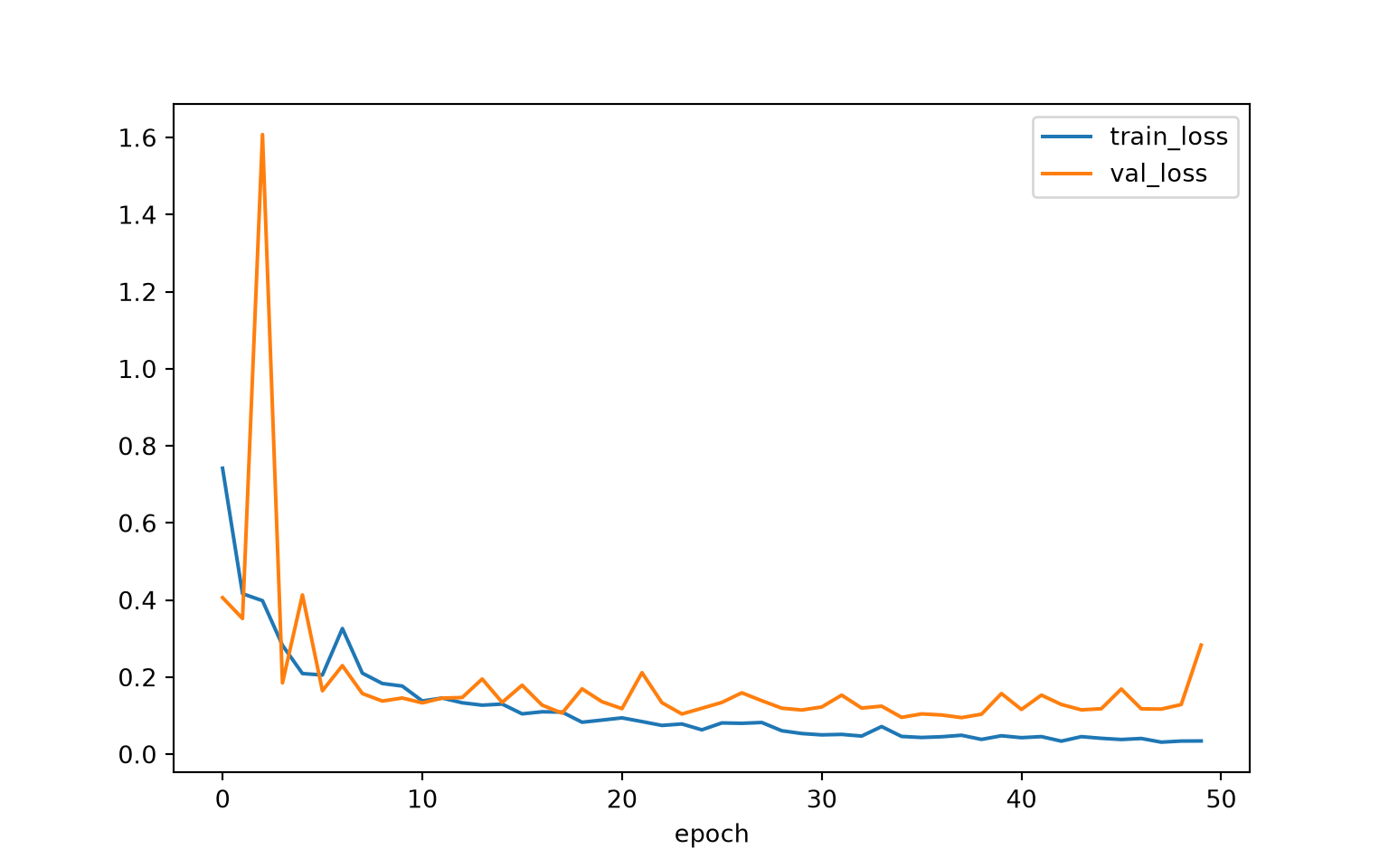
plt.rcParams['figure.figsize'] = [10, 10]
firstPlot = resultsDF.plot(x='epoch', y="train_f1")
resultsDF.plot(x='epoch', y="val_f1", ax=firstPlot)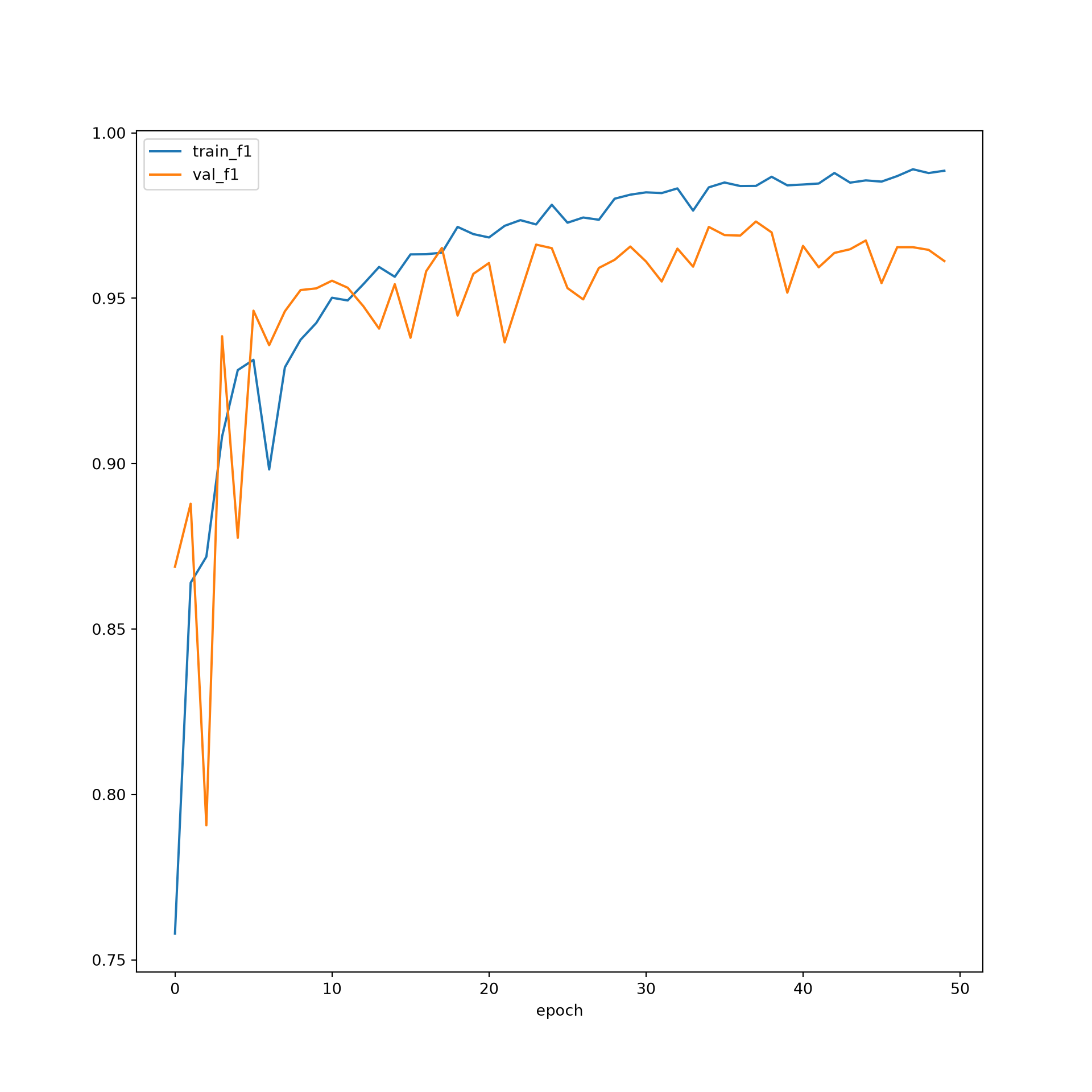
13.5 Using Different Learning Rates for Different Stages
When a model is initialized using pre-trained parameters, not all components of the model are in the same state. In our modified ResNet-34, the first convolutional and batch normalization layers and the final fully connected layer were replaced, so they were initialized with random parameters. The remaining layers start from parameters learned from ImageNet. Further, the layers within a CNN learn features at different levels of abstraction. The early layers learn general, low-level features, such as edges, textures, and color gradients, which tend to be useful for many tasks, while the later layers learn more complex, task-specific features. As a result, it is common to update the pre-trained layers more gently than the randomly initialized layers and to update the early pre-trained layers more gently than the later ones. Using a single, large learning rate for all layers risks quickly destroying the useful pre-trained features, a problem sometimes called catastrophic forgetting, while using a single, small learning rate may be too slow for the randomly initialized layers.
Using different learning rates for different components of a model is known as discriminative learning rates or layer-wise learning rates. As noted in Chapter 21, I have generally found that using lower learning rates for the pre-trained encoder stabilizes the training process when fine-tuning.
Howard, J. and Ruder, S., 2018. “Universal language model fine-tuning for text classification.” In Proceedings of the 56th Annual Meeting of the Association for Computational Linguistics (pp. 328-339).
In PyTorch, different learning rates are implemented using parameter groups. Instead of passing all of the model’s parameters to the optimizer, you pass a list of dictionaries. Each dictionary contains a "params" key, which lists the parameters in the group, and an "lr" key, which defines the learning rate for that group. Any other optimizer setting, such as weight decay, can also be set separately for each group. Here, I also include a "name" key, which is ignored by the optimizer but used by Lightning’s LearningRateMonitor callback to label the logged learning rates.
The torchvision ResNet is organized into the following components, which define the stages of the network:
-
conv1,bn1: the stem, which I replaced and is therefore randomly initialized. -
layer1throughlayer4: the four stages of residual blocks, which are pre-trained. -
fc: the final fully connected layer, which I replaced and is therefore randomly initialized.
The function below creates the parameter groups. The stem and head receive the full base learning rate since they are randomly initialized. The four residual stages receive smaller learning rates, with the earliest stage receiving the smallest. The lrMult argument defines the multiplier applied to the base learning rate for each of the four stages.
def resnetParamGroups(model, baseLR=1e-3, lrMult=(0.01, 0.03, 0.1, 0.3)):
    return [
        {"params": list(model.conv1.parameters()) + list(model.bn1.parameters()),
         "lr": baseLR, "name": "stem"},
        {"params": model.layer1.parameters(), "lr": baseLR*lrMult[0], "name": "layer1"},
        {"params": model.layer2.parameters(), "lr": baseLR*lrMult[1], "name": "layer2"},
        {"params": model.layer3.parameters(), "lr": baseLR*lrMult[2], "name": "layer3"},
        {"params": model.layer4.parameters(), "lr": baseLR*lrMult[3], "name": "layer4"},
        {"params": model.fc.parameters(), "lr": baseLR, "name": "head"},
    ]
To use the parameter groups with Lightning, I subclass LitClassifier and override its configure_optimizers() method. Every parameter in the model must belong to exactly one group; if a parameter is listed in two groups, PyTorch will raise an error, and if it is not listed in any group, it will not be updated.
class LitTransfer(LitClassifier):
    def __init__(self, model, nCls, lr=1e-3, lrMult=(0.01, 0.03, 0.1, 0.3)):
        super().__init__(model, nCls, lr)
        self.lrMult = lrMult

    def configure_optimizers(self):
        groups = resnetParamGroups(self.model, self.lr, self.lrMult)
        return torch.optim.AdamW(groups)

model = initialize_model(resNet="34", nChn=10, nCls=10, freeze=False, pretrained=True)
litTransfer = LitTransfer(model, nCls=10, lr=1e-3)
13.5.1 Adjusting Learning Rates During Training
The learning rates for each group can also change during training. There are two common approaches: (1) applying a learning rate scheduler, which modifies the learning rate of every group, and (2) gradual unfreezing, in which the pre-trained stages are frozen initially and unfrozen during training.
13.5.1.1 Schedulers with Parameter Groups
Learning rate schedulers operate on all of the parameter groups in an optimizer. Some schedulers, such as OneCycleLR, accept a list of maximum learning rates, one for each group. In the example below, the one cycle policy, which was introduced in Chapter 7, is applied to every group, but each group follows its own schedule with its own maximum learning rate. The relative differences between the stages are maintained throughout training. The LearningRateMonitor callback logs the learning rate of each group so that the schedules can be checked.
class LitTransferOneCycle(LitTransfer):
    def configure_optimizers(self):
        groups = resnetParamGroups(self.model, self.lr, self.lrMult)
        optimizer = torch.optim.AdamW(groups)
        scheduler = torch.optim.lr_scheduler.OneCycleLR(
            optimizer,
            max_lr=[g["lr"] for g in groups],
            total_steps=self.trainer.estimated_stepping_batches)
        return {"optimizer": optimizer,
                "lr_scheduler": {"scheduler": scheduler, "interval": "step"}}

litTransfer = LitTransferOneCycle(model, nCls=10, lr=1e-3)
trainer = L.Trainer(max_epochs=50, accelerator="gpu", devices=1, precision="bf16-mixed",
                    default_root_dir="data/output/",
                    callbacks=[checkpoint, LearningRateMonitor(logging_interval="step")])
13.5.1.2 Gradual Unfreezing
With gradual unfreezing, the pre-trained layers are frozen at the beginning of training so that only the randomly initialized stem and head are updated. Once these layers have adapted to the pre-trained features, the pre-trained stages are unfrozen, often one at a time starting from the last stage, and added to the training process with small learning rates. This prevents the large, noisy gradients produced by the randomly initialized layers early in training from disrupting the pre-trained parameters.
Lightning implements this using the BaseFinetuning callback. Subclasses define two methods. The freeze_before_training() method freezes the specified modules before training begins. The finetune_function() method is called at the start of each epoch and can unfreeze modules and add their parameters to the optimizer as a new parameter group with a specified learning rate using unfreeze_and_add_param_group(). Since the frozen stages are not passed to the optimizer at the beginning of training, configure_optimizers() must only include the trainable parameters. In the example, layer4 is unfrozen at the start of epoch 3, layer3 at epoch 5, and layer1 and layer2 at epoch 7, each with a learning rate that is a fraction of the base learning rate.
class GradualUnfreeze(BaseFinetuning):
    def __init__(self, baseLR=1e-3):
        super().__init__()
        self.baseLR = baseLR

    def freeze_before_training(self, pl_module):
        m = pl_module.model
        self.freeze([m.layer1, m.layer2, m.layer3, m.layer4])

    def finetune_function(self, pl_module, current_epoch, optimizer):
        m = pl_module.model
        if current_epoch == 3:
            self.unfreeze_and_add_param_group(m.layer4, optimizer, lr=self.baseLR*0.3)
        elif current_epoch == 5:
            self.unfreeze_and_add_param_group(m.layer3, optimizer, lr=self.baseLR*0.1)
        elif current_epoch == 7:
            self.unfreeze_and_add_param_group([m.layer1, m.layer2], optimizer, lr=self.baseLR*0.02)

class LitTransferUnfreeze(LitClassifier):
    def configure_optimizers(self):
        trainable = [p for p in self.parameters() if p.requires_grad]
        return torch.optim.AdamW(trainable, lr=self.lr)

litTransfer = LitTransferUnfreeze(model, nCls=10, lr=1e-3)
trainer = L.Trainer(max_epochs=50, accelerator="gpu", devices=1, precision="bf16-mixed",
                    default_root_dir="data/output/",
                    callbacks=[GradualUnfreeze(baseLR=1e-3), checkpoint,
                               LearningRateMonitor(logging_interval="epoch")])
trainer.fit(litTransfer, train_dataloaders=trainDL, val_dataloaders=valDL)
Note that freezing modules that contain batch normalization layers also stops their running means and variances from being updated, since BaseFinetuning places frozen modules in evaluation mode. Lightning also provides a BackboneFinetuning callback, which implements a common version of this strategy for LightningModules that store their pre-trained component as a backbone attribute.
13.5.1.3 Manually Adjusting Learning Rates
Lastly, the learning rate of any parameter group can be changed at any time by editing the "lr" value in the optimizer’s param_groups list. In the example below, a simple callback multiplies the learning rate of every pre-trained stage by 0.5 every 10 epochs while leaving the stem and head unchanged. This approach offers complete flexibility, although for most purposes one of the schedulers provided by PyTorch is sufficient.
class HalvePretrainedLR(L.Callback):
    def on_train_epoch_start(self, trainer, pl_module):
        epoch = trainer.current_epoch
        if epoch > 0 and epoch % 10 == 0:
            optimizer = trainer.optimizers[0]
            for g in optimizer.param_groups:
                if g.get("name", "").startswith("layer"):
                    g["lr"] = g["lr"] * 0.5
Which strategy works best depends on the problem, the size of the training dataset, and how different the new data are from the data used to pre-train the model. In this example, the EuroSAT data differ substantially from ImageNet: they have 10 spectral bands as opposed to 3, a spatial resolution of 10 m, and an overhead perspective. In such cases, the pre-trained parameters generally need to change more, so freezing the encoder for the entire training process is not recommended, but lower learning rates for the early stages can still help stabilize training. When the new data are more similar to the pre-training data and the training dataset is small, keeping more of the network frozen may be preferable.
13.6 Model Assessment
I next assess the model using the withheld test data. I re-instantiate the architecture and pass it to load_from_checkpoint(), which restores the saved parameters from the Lightning checkpoint file. Since the model argument was excluded from the saved hyperparameters, it must be provided when the checkpoint is loaded. I then define a DataSet and DataLoader for the testing samples, and call the test() method of a Trainer. The testing samples are normalized using the band means and standard deviations of the training data, and no data augmentations are applied. If you trained a model above, you can instead use ckpt_path="best".
model = initialize_model(resNet="34", nChn=10, nCls=10, freeze=False, pretrained=False)
litModel = LitClassifier.load_from_checkpoint("data/models/resnetEurosatVariable.ckpt",
                                              model=model, map_location="cpu")

testDS = EuroSat(test, mnImg, sdImg, transform=None)
testDL = torch.utils.data.DataLoader(testDS, batch_size=32, shuffle=False, num_workers=0)

trainer = L.Trainer(accelerator="gpu", devices=1, logger=False)
testResults = trainer.test(litModel, dataloaders=testDL)
The results look pretty good. I achieved an overall accuracy greater than 97% for predicting to new data.
The class-level assessment metrics are obtained below using the predicted class probabilities returned by the predict() method.
probs = torch.cat(trainer.predict(litModel, dataloaders=testDL))
targets = torch.tensor(test.iloc[:len(probs), 3].to_numpy()).long()

cm = tm.ConfusionMatrix(task="multiclass", num_classes=10)
f1 = tm.F1Score(task="multiclass", num_classes=10, average="none")
precision = tm.Precision(task="multiclass", num_classes=10, average="none")
recall = tm.Recall(task="multiclass", num_classes=10, average="none")

print(cm(probs, targets))
print(f1(probs, targets))
print(precision(probs, targets))
print(recall(probs, targets))
13.7 Concluding Remarks
The goal of this chapter was to explore the use of transfer learning by initializing a model architecture using parameters/weights learned from a prior dataset, in this case ImageNet, as opposed to initializing the model parameters randomly. Since this was a very different problem, I did not freeze any of the model parameters/weights. Instead, all parameters were updated during the learning process, but starting from the pre-trained parameters/weights as opposed to a random initialization. We also explored using PyTorch Lightning to apply different learning rates to different stages of the model and to adjust these learning rates during training using schedulers, gradual unfreezing, and callbacks.
Transfer learning can be a very powerful technique, especially when your training dataset is not large. These methods are especially useful when you are using a common architecture, such as VGGNet-16 or a ResNet architecture, that has already been trained using a large dataset. As you will see in the semantic segmentation sections, these architectures, pre-trained models, and transfer learning can be used in the encoder component of semantic segmentation models. So, we will continue to explore these techniques throughout the next set of chapters relating to semantic segmentation.
13.8 Questions
- Define transfer learning. Why might transfer learning allow a model to be trained using fewer training samples?
- Describe three options for using pre-trained weights in the convolutional component of a CNN architecture. Explain how gradual unfreezing combines these options during training.
- Why were none of the model parameters frozen when training the ResNet-34 architecture to classify the EuroSAT data in this chapter?
- Which components of the modified ResNet-34 architecture were not initialized using the ImageNet weights, and why?
- The ImageNet weights were learned from three-band RGB photographs, while the EuroSAT data used in this chapter have ten spectral bands. What challenges does this create when applying transfer learning to multispectral data?
- Compare the number of trainable parameters and the test set performance of the ResNet-34 model trained in this chapter to those of the CNN trained from scratch in Chapter 11.
- Explain why it is common to use lower learning rates for the pre-trained stages of a model than for randomly initialized components, and lower learning rates for early stages than for later stages. How are different learning rates implemented in PyTorch using parameter groups?
- Design an experiment to assess whether freezing the convolutional component of a pre-trained ResNet-34 architecture impacts model performance for the EuroSAT classification problem. What settings should be held constant between the compared models, and what metrics would you use to compare them?
13.9 Exercises
The exercise for this part of the text is the midterm project described in Chapter 14.