7  Improving Models

7.1 Introduction

In its current state, deep learning is science, art, and tradecraft. As a result, analysts learn with time and experience what techniques may help them achieve more accurate and generalizable models. Unfortunately, due to the complexity of these models and the methods used to train them, it is not possible to assess all possible options to potentially improve models. Instead, individuals must build intuition as to what methods might be most appropriate for their specific use case or application domain. With that said, there are some commonly used techniques that are often explored, and those are the focus of this chapter. Note that I am saving a discussion of some specific methods, such as transfer learning and architecture modifications, for later chapters.

Methods that are often explored to potentially improve model performance include the following.

1. Collecting more or better training data. Deep learning models tend to be data hungry, partially due to the large number of parameters that must be estimated and the issue of overfitting. As a result, adding training samples is an often first suggestion to improve model performance. Unfortunately, it is not always practical or possible to collect more data. Further, the number of samples that are needed to successfully train a model without overfitting is not generally clearly defined. This is often case specific.
2. It is possible to initialize models using weights/parameters learned from other datasets. For example, large datasets, such as ImageNet and Common Objects in Context (COCO), can be used to train models. The learned parameters can be used as a starting point to then apply the model to a new problem or dataset. This can be accomplished by initializing the model using these learned parameters but still training the entire architecture, essentially using these parameters as a starting point as opposed to using a random initialization. When learned parameters are used to initialized the model but all components are still trainable or updateable, it has been documented that using different learning rates for different components of the architecture can be useful. We will discuss this in Chapter 13. Another option when applying pre-trained parameters is to only train part of the architecture, essentially leaving part of the architecture frozen or untrainable. The assumption is that the learned parameters may be adequate enough for the current task or that they capture information that is meaningful for the new task to which they are being applied. The process of using parameters that were learned from another, and often much larger, dataset is called transfer learning. We will discuss transfer learning in Chapter 13, so will not cover it in this chapter.
3. In order to reduce overfitting and improve model generalization, it is common to augment the input data. Using images as an example, random flips, rotations, sharpening, blurring, and/or adjustments to saturation, contrast, and/or brightness can be applied. This is termed image augmentation, and the idea is that creating more variability in the training data can result in a more varied representation and thus discourage overfitting to the training data. Data augmentation using the Albumentations package was discussed in Chapter 5, and we will apply augmentations when training CNNs for scene labeling and semantic segmentation in later chapters.
4. Data imbalance can have a negative impact on the learning process. Classes that make up a larger proportion of the training dataset will have a larger impact on the learning process and the calculated loss; as a result, the model will tend to focus more on these classes as opposed to less abundant classes. Practically, this can result in the model doing a poorer job at predicting the less abundant classes, overpredicting the abundance of the more prominent classes, and/or underpredicting the abundance of the less prominent classes. There are several methods to combat overfitting including using class weightings in the loss metric calculations, using loss metrics that are less impacted by class imbalance, and/or augmenting the training data so that classes are represented with more even abundance. We will discuss these methods in this section.
5. The model architecture can also be altered to potentially improve model performance. Common modifications include integrating batch normalization and/or dropouts, increasing the complexity of the network so that it can model more complex patterns in the data, and using different activation functions, such as leaky ReLU, Swish, or GELU. We will discuss some of these methods in this chapter. One issue here is that increasing the complexity of the network can result in overfitting and reduced generalization, especially if the training dataset is small. Thus, increasing the size and complexity of the model architecture may not have the desired effect. A lot of convolutional neural network architectures have been specifically designed and proposed to deal with the issue of capturing complex patterns while not overfitting to the training dataset. We will discuss some of these architectures and logic behind them in later sections.
6. The optimization algorithm used can have a large impact on the modeling process, and there are many alternatives to traditional mini-batch stochastic gradient descent that are derived from and build on this method. I generally use the AdamW optimizer as a default. However, people have varying opinions about the best optimizer for a specific use case. They all have pros and cons.
7. Regardless of the optimizer used, the selected learning rate can have a large impact on model performance. My go-to first attempts to potentially improve model performance are (1) to change or augment the loss function being used and/or (2) to adjust the learning rate. There are other optimizer-specific settings that can impact the learning process as well. One means to select the learning rate specifically is to make use of a learning rate finder. We will discuss learning rate finders in this chapter.
8. It is possible to augment the learning rate, or other parameter settings, during the learning process. In PyTorch this is generally implemented using schedulers or callbacks. We will explore schedulers in this section.
9. There are other training loop modifications that may also be helpful. In this chapter, we will explore gradient accumulation.
10. Modifying the targets used to calculate the loss can reduce overconfidence and the impact of label noise. We will explore label smoothing in this chapter.
11. Lastly, when experimenting with these methods, it is useful to be able to reproduce a training process. We will discuss the settings required to make PyTorch training reproducible.

7.2 Preparation

As normal, I begin with imports. I also set the device variable. Here, I am specifically making use of a GPU to potentially speed up computation.

import numpy as np
import pandas as pd
import matplotlib
from matplotlib import pyplot as plt
import seaborn as sns
plt.rcParams['figure.figsize'] = [20, 20]

import os
import random

from sklearn.utils.class_weight import compute_class_weight

import torch
import torch.nn as nn
import torch.nn.functional as F
from torch.utils.data.dataset import Dataset
from torch.utils.data import DataLoader

import torchmetrics as tm

device = torch.device("cuda:0" if torch.cuda.is_available() else "cpu")
print(device)

cuda:0

I will use the same data and problem that we have been exploring: the differentiation of land cover types using band means derived from the EuroSatAllBands dataset. There is nothing new in the code blocks below. Here is a quick review of the data preparation process.

1. Read in the data tables of band means
2. Calculate the means and standard deviations from the training dataset
3. Define a DataSet subclass
4. Instantiate the datasets and normalize the band means
5. Instantiate the DataLoaders

trainAgg = pd.read_csv("data/files/EuroSat_Tabulated/train_aggregated.csv")
testAgg = pd.read_csv("data/files/EuroSat_Tabulated/test_aggregated.csv")
valAgg = pd.read_csv("data/files/EuroSat_Tabulated/val_aggregated.csv")

trainAgg.head()

   Unnamed: 0       class  code  ...  NIR_Narrow        swir1        swir2
0           0  AnnualCrop     0  ...  674.346680  1461.915527  3229.570801
1           1  AnnualCrop     0  ...  758.629395  1189.456543  2714.708008
2           2  AnnualCrop     0  ...  761.717041  1621.122070  3900.247314
3           3  AnnualCrop     0  ...  638.532471  1469.149170  3986.078125
4           4  AnnualCrop     0  ...  948.018066  1656.648682  3609.164551

[5 rows x 13 columns]

trainAggMns = np.array(trainAgg.iloc[:,3:].mean(axis=0)).flatten()
print(trainAggMns)

[1116.07645724 1035.31213955  937.87729602 1184.29159721 1971.09456594
 2334.38145703 2262.04021603  724.95266414 1103.83350066 2552.01787743]

trainAggSDs = np.array(trainAgg.iloc[:,3:].std(axis=0)).flatten()
print(trainAggSDs)

[ 255.54328897  312.29876238  479.85770488  500.93361557  779.66575883
  976.84613356  970.08515215  384.49257895  670.88688372 1120.89990655]

class EuroSat(Dataset):

    def __init__(self, df, bndMns, bndSDs):
        super().__init__
        self.df = df
        self.bndMns = bndMns
        self.bndSDs = bndSDs

    def __getitem__(self, idx):
        bands = [self.df.iloc[idx, 3:]]
        label = [self.df.iloc[idx, 2]]
        bands = np.array(bands)
        bands = (bands-self.bndMns)/self.bndSDs
        label = np.array(label)
        bands = bands.astype('float32')
        bands = torch.from_numpy(bands).squeeze().float()
        label = torch.from_numpy(label).squeeze().float()
        label = label.long()
        return bands, label

    def __len__(self):
        return len(self.df)

trainDS = EuroSat(trainAgg, trainAggMns, trainAggSDs)
testDS = EuroSat(testAgg, trainAggMns, trainAggSDs)
valDS = EuroSat(valAgg, trainAggMns, trainAggSDs)

trainDL = torch.utils.data.DataLoader(trainDS, batch_size=256, shuffle=True, sampler=None,
num_workers=0, pin_memory=False, drop_last=False)
testDL = torch.utils.data.DataLoader(testDS, batch_size=256, shuffle=True, sampler=None,
num_workers=0, pin_memory=False, drop_last=False)
valDL = torch.utils.data.DataLoader(valDS, batch_size=256, shuffle=True, sampler=None,
num_workers=0, pin_memory=False, drop_last=False)

7.3 Dropouts

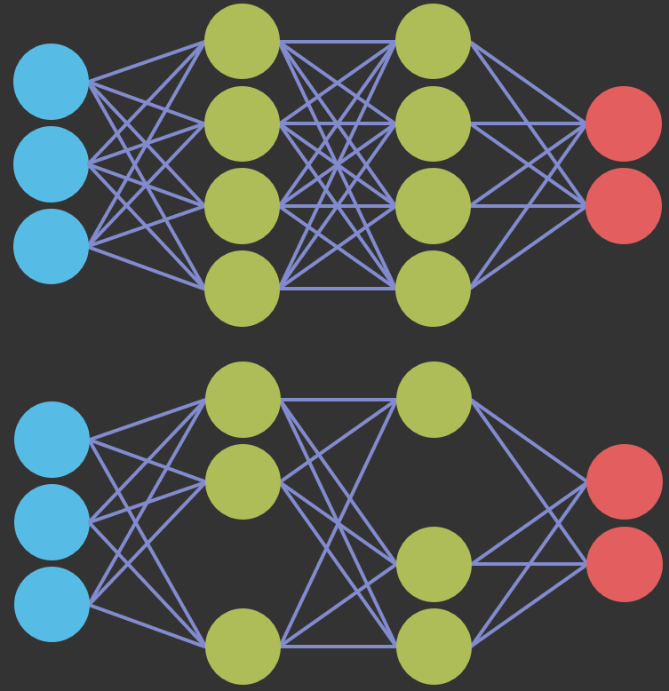
Dropouts are a regularization method in which certain neurons are dropped out or their associated parameters are not updated within the training loop during passes over training mini-batches. The idea is that not updating all of the weights/parameters during each weight update can result in reduced overfitting and improved generalization. How many neurons will be dropped in each weight update is controlled by the p parameter. In the example model architecture below, I am applying dropouts between each fully connected layer, which will cause a random 30% of the neurons to not be updated with each weight/parameter update. Note that I do not use dropouts after the final fully connected layer. Dropouts are implemented in PyTorch using nn.Dropout().

Dropouts are conceptualized in Figure 7.1. A different random subset of neurons is dropped for each mini-batch, so the network cannot rely too heavily on any single neuron or connection. Dropouts are only applied during training. When the model is placed in evaluation mode using model.eval(), all neurons are used. To keep the magnitude of the activations consistent between training and inference, PyTorch scales the outputs of the retained neurons by \(\frac{1}{1-p}\) during training.

Figure 7.1. Dropouts. The top network is fully connected, while, in the bottom network, a random subset of the hidden layer neurons and their associated connections have been dropped for a training mini-batch.

There is currently some debate as to whether dropouts are still necessary or useful. With the advent and wide adoption of batch normalization, dropouts have generally been used less frequently. Analysts are using batch normalization as a means to potentially reduce overfitting and improve generalization as opposed to dropouts, and including both dropouts and batch normalization may be unnecessary. Again, analysts have varying opinions. I generally prefer to use batch normalization as opposed to dropouts. However, you may want to experiment with dropouts as a potential means to improve model performance. Note that dropout methods are also available for convolutional layers.

class myFCNDrop(nn.Module):
  def __init__(self, inSize, hiddenSizes, outSize):
    super().__init__()
    self.inSize = inSize
    self.hiddenSize = hiddenSizes
    self.outSize = outSize

    self.theNetwork = nn.Sequential(
        nn.Linear(inSize, hiddenSizes[0]),
        nn.Dropout(p=0.3),
        nn.ReLU(inplace=True),
        nn.Linear(hiddenSizes[0], hiddenSizes[1]),
        nn.Dropout(p=.3),
        nn.ReLU(inplace=True),
        nn.Linear(hiddenSizes[1], outSize)
    )

  def forward(self, x):
    x = self.theNetwork(x)
    return x

7.4 Alternative Activation Functions

The rectified linear unit (ReLU) has been the default activation function in deep learning for many years. It is simple and fast to compute, and since its gradient is 1 for all positive inputs, it alleviates the vanishing gradient problem associated with older activation functions, such as the sigmoid and hyperbolic tangent, whose gradients approach zero for large positive or negative inputs. However, several alternatives have been proposed that can improve model performance, and they are now commonly used in modern architectures. In this section, I discuss three alternatives: leaky ReLU, Swish (also called SiLU), and the Gaussian error linear unit (GELU). The definitions are summarized in Table 7.1, where \(\Phi(x)\) is the cumulative distribution function of the standard normal distribution and \(\sigma(x)\) is the sigmoid function.

Table 7.1. Comparison of activation functions.

Activation	Definition	PyTorch	Trainable parameters
ReLU	\(\max(0, x)\)	nn.ReLU()	None
Leaky ReLU	\(x\) if \(x > 0\); \(a x\) otherwise	nn.LeakyReLU(negative_slope=a)	None
Swish/SiLU	\(x \cdot \sigma(x)\)	nn.SiLU()	None
GELU	\(x \cdot \Phi(x)\)	nn.GELU()	None

7.4.1 Leaky ReLU

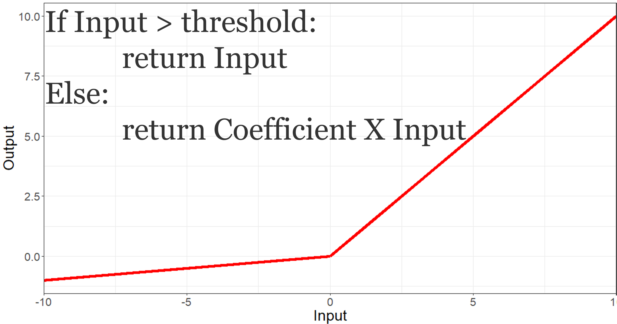
One known issue with ReLU is the problem of “dying ReLU”. Remember that this activation function works by converting negative activations to 0 and maintaining all positive activation values. If a neuron’s inputs are such that its pre-activation values are negative for all samples, its output will always be 0. This will result in a gradient of 0, so the weights feeding into that neuron will no longer be updated, and the neuron effectively “dies”. This can happen, for example, after a large parameter update caused by a high learning rate. To alleviate this issue, the leaky ReLU was introduced. Instead of simply converting all negative activations to 0, negative values are maintained but with a reduced magnitude by multiplying them by a slope term that is less than 1. As a result, a small gradient is maintained for negative inputs. Leaky ReLU is shown in Figure 7.2.

Figure 7.2. The leaky ReLU activation function. Positive inputs are returned unchanged, and negative inputs are multiplied by a small coefficient, or negative slope, so that they are not converted to 0.

In PyTorch, ReLU can be replaced with leaky ReLU by simply changing nn.ReLU() to nn.LeakyReLU(). You can also set the negative slope parameter, which is 0.01 by default.

I have generally found using leaky ReLU to be useful and worth considering. It is a very simple change, and it does not add trainable parameters to the model. There are also versions of ReLU that introduce trainable parameters, such as the parametric ReLU (PReLU), in which the negative slope is learned during training.

class myFCNLeaky(nn.Module):
  def __init__(self, inSize, hiddenSizes, outSize):
    super().__init__()
    self.inSize = inSize
    self.hiddenSize = hiddenSizes
    self.outSize = outSize

    self.theNetwork = nn.Sequential(
        nn.Linear(inSize, hiddenSizes[0]),
        nn.BatchNorm1d(hiddenSizes[0]),
        nn.LeakyReLU(negative_slope=0.1, inplace=True),
        nn.Linear(hiddenSizes[0], hiddenSizes[1]),
        nn.BatchNorm1d(hiddenSizes[1]),
        nn.LeakyReLU(negative_slope=0.1, inplace=True),
        nn.Linear(hiddenSizes[1], outSize)
    )

  def forward(self, x):
    x = self.theNetwork(x)
    return x

7.4.2 Swish (SiLU)

The Swish activation function was identified by Ramachandran et al. (2017) using an automated search over possible activation functions. It is defined as the input multiplied by the sigmoid of the input, \(x \cdot \sigma(x)\). In PyTorch, it is implemented as nn.SiLU(), since the same function was earlier described as the sigmoid-weighted linear unit (SiLU). Swish differs from ReLU in several ways:

1. It is smooth: unlike ReLU, which has an abrupt change in slope at 0, Swish is differentiable everywhere. Smooth activation functions can result in a smoother loss surface, which may make optimization easier.
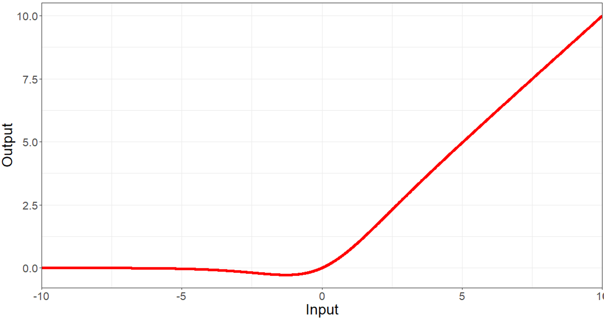
2. It is non-monotonic: for negative inputs, the output first decreases and then increases toward 0, with a minimum value of approximately -0.28. So, small negative values are maintained while large negative values are suppressed.
3. It does not completely zero out negative inputs, so it avoids the dying ReLU problem.

These characteristics can be observed in Figure 7.3.

Figure 7.3. The Swish (SiLU) activation function. The function is smooth and non-monotonic: the output dips slightly below 0 for small negative inputs before approaching 0 for large negative inputs.

Swish is used in several modern architectures, including the EfficientNet family of CNNs. The main disadvantage relative to ReLU is that it is slightly more computationally expensive since it requires calculating the sigmoid function.

Ramachandran, P., Zoph, B. and Le, Q.V., 2017. “Searching for activation functions.” arXiv preprint arXiv:1710.05941.

7.4.3 Gaussian Error Linear Unit (GELU)

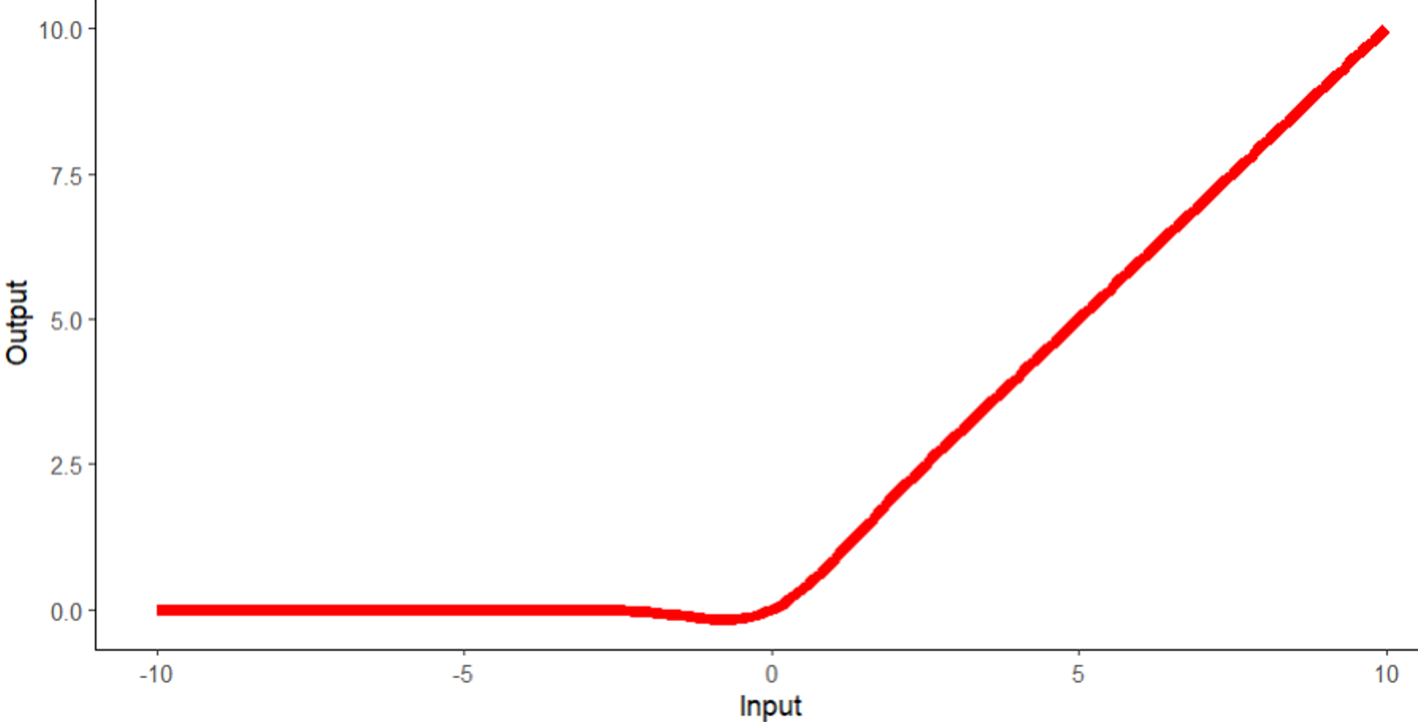
The Gaussian error linear unit (GELU), proposed by Hendrycks and Gimpel (2016), multiplies the input by the probability that a standard normal random variable is less than the input, \(x \cdot \Phi(x)\). Conceptually, it can be thought of as weighting each input by its value as opposed to gating it by its sign, as ReLU does: large positive inputs are passed through nearly unchanged, large negative inputs are suppressed to nearly 0, and inputs near 0 are partially passed. GELU is very similar in shape to Swish; both are smooth, non-monotonic, and allow small negative values. In fact, GELU is closely approximated by \(x \cdot \sigma(1.702x)\). Compare Figure 7.4 with Figure 7.3.

Figure 7.4. The Gaussian error linear unit (GELU) activation function. Similar to Swish, GELU is smooth and non-monotonic, but its dip below 0 is narrower and shallower.

GELU is the default activation function in transformer architectures, including BERT, the GPT models, and the Vision Transformer, and it is used in ConvNeXt, which we will explore in Chapter 24. PyTorch provides nn.GELU(), and setting approximate="tanh" uses a faster approximation based on the hyperbolic tangent function.

Hendrycks, D. and Gimpel, K., 2016. “Gaussian error linear units (GELUs).” arXiv preprint arXiv:1606.08415.

7.4.4 Comparing Activation Functions

The code below plots each activation function and its gradient. The gradients are calculated using automatic differentiation by setting requires_grad=True for the input tensor, summing the output, and calling backward(). Note that the ReLU gradient changes abruptly from 0 to 1 at an input of 0, the leaky ReLU gradient is a small positive value for negative inputs, and the Swish and GELU gradients change smoothly and are slightly negative for some negative inputs.

acts = {"ReLU": nn.ReLU(), "Leaky ReLU": nn.LeakyReLU(0.1),
        "Swish/SiLU": nn.SiLU(), "GELU": nn.GELU()}

fig, axs = plt.subplots(1, 2, figsize=(11, 4))
for name, act in acts.items():
    x = torch.linspace(-5, 5, 501, requires_grad=True)
    y = act(x)
    y.sum().backward()
    axs[0].plot(x.detach(), y.detach(), label=name)
    axs[1].plot(x.detach(), x.grad, label=name)
axs[0].set_title("Activation")
axs[1].set_title("Gradient")
for ax in axs:
    ax.axhline(0, color="gray", linewidth=0.5)
    ax.axvline(0, color="gray", linewidth=0.5)
    ax.legend()
plt.show()

To make it easy to experiment with different activation functions, the activation can be passed as a parameter when defining an architecture. In the example below, the user provides a string that is mapped to the appropriate PyTorch layer. This is the approach used in the customizable UNet architecture that we build in Chapter 18.

def makeAct(actFunc="relu", negative_slope=0.01):
    if actFunc == "lrelu":
        return nn.LeakyReLU(negative_slope=negative_slope, inplace=True)
    elif actFunc == "swish":
        return nn.SiLU(inplace=True)
    elif actFunc == "gelu":
        return nn.GELU()
    return nn.ReLU(inplace=True)

class myFCNAct(nn.Module):
  def __init__(self, inSize, hiddenSizes, outSize, actFunc="relu"):
    super().__init__()
    self.theNetwork = nn.Sequential(
        nn.Linear(inSize, hiddenSizes[0]),
        nn.BatchNorm1d(hiddenSizes[0]),
        makeAct(actFunc),
        nn.Linear(hiddenSizes[0], hiddenSizes[1]),
        nn.BatchNorm1d(hiddenSizes[1]),
        makeAct(actFunc),
        nn.Linear(hiddenSizes[1], outSize)
    )

  def forward(self, x):
    return self.theNetwork(x)

model = myFCNAct(10, [256, 256], 10, actFunc="gelu").to(device)

Which activation function should you use? ReLU remains a strong and efficient default, especially for CNNs. However, I have found that leaky ReLU, Swish, and GELU are worth experimenting with since they are simple changes that do not add trainable parameters. Swish and GELU tend to perform similarly to each other; GELU is the standard choice for transformer-based architectures and modern CNNs inspired by them, while Swish is common in efficient CNN architectures. Note that changing the activation function may also require adjusting the learning rate, and the benefits are generally modest relative to changes to the data, loss function, or learning rate.

7.5 Class Weighting

One means to potentially reduce the impact of class imbalance in the dataset is to apply weights to each class when performing the loss calculations. Specifically, less abundant classes should have a higher weight in the loss calculation in comparison to more abundant classes. To accomplish this, it is common to calculate weights as the inverse of their relative abundance in the dataset.

Fortunately, scikit-learn provides the compute_class_weight() function for accomplishing this. This requires to first extract the class labels into a NumPy array. Setting the class_weight parameter to ‘balanced’ will yield weights that equalize the impact of each class on the weight updates. Once the weights are defined, they can be written to a torch tensor and moved to the device.

Some loss metrics allow for the incorporation of class weights. Here, I have provided an example of defining a cross entropy loss with class weights using the weight parameter in the nn.CrossEntropyLoss() implementation. To see if weights can be used and how they are integrated using other loss functions, please consult the associated documentation.

It is also possible to incorporate class weights into some assessment metric calculations. Although this won’t inform the parameter updates, it can be useful for selecting a model or determining whether the model is improving.

npLbls = np.array(trainAgg.iloc[:,3])

npLbls

array([1301.21630859, 1042.02490234, 1411.48461914, ...,  963.27075195,
       1153.65087891, 1105.24951172], shape=(16558,))

weights = compute_class_weight(class_weight='balanced', classes=np.unique(npLbls), y=npLbls)
weightsT = torch.tensor(weights,dtype=torch.float).to(device)

weightsT

tensor([1.0025, 1.0025, 1.0025,  ..., 1.0025, 1.0025, 1.0025], device='cuda:0')

criterion = nn.CrossEntropyLoss(weight=weightsT).to(device)

7.6 Label Smoothing

When training a classifier with cross entropy loss, the reference labels are represented as one-hot encodings: the correct class has a target probability of 1 and all other classes have a target probability of 0. To fully minimize the loss, the model must predict a probability of exactly 1 for the correct class, which requires the logit for the correct class to become infinitely larger than the other logits. As a result, the model is continually pushed toward larger logits and more extreme, overconfident predictions. This can contribute to overfitting and results in predicted probabilities that do not reflect the model’s actual uncertainty, which is a problem if you plan to use the probabilities, for example, to map the likelihood of a class or to set a decision threshold.

Label smoothing (Szegedy et al., 2016) addresses this by softening the targets. With a smoothing factor of \(\varepsilon\) and \(K\) classes, the target probability for the correct class becomes \(1 - \varepsilon + \varepsilon/K\), and the target probability for each other class becomes \(\varepsilon/K\). For example, with \(\varepsilon = 0.1\) and 10 classes, the correct class has a target of 0.91 and each other class has a target of 0.01. Since the targets are no longer 0 and 1, the loss is minimized by finite logits, so the model is discouraged from becoming overconfident.

Label smoothing can also reduce the impact of label noise, or incorrect reference labels, which is common in geospatial datasets generated by manual interpretation or derived from existing maps. Since the model is never asked to be completely certain, a small number of mislabeled samples has less influence on the parameter updates.

In PyTorch, label smoothing is built into nn.CrossEntropyLoss() via the label_smoothing argument. Values between 0.05 and 0.2 are common. It can also be combined with class weights.

criterion = nn.CrossEntropyLoss(label_smoothing=0.1).to(device)

# Combined with class weights
criterion = nn.CrossEntropyLoss(weight=weightsT, label_smoothing=0.1).to(device)

To see how label smoothing changes the targets, the code below manually converts a set of class indices to smoothed target distributions. Since nn.CrossEntropyLoss() also accepts class probabilities as targets, providing these smoothed targets with no label_smoothing argument yields the same loss as providing the class indices with label_smoothing=0.1.

eps = 0.1
nCls = 10
labels = torch.tensor([0, 3, 7])
smoothed = F.one_hot(labels, nCls).float() * (1 - eps) + eps / nCls
print(smoothed)

logits = torch.randn(3, nCls)
print(nn.CrossEntropyLoss(label_smoothing=eps)(logits, labels))
print(nn.CrossEntropyLoss()(logits, smoothed))

There are a few things to keep in mind when using label smoothing. First, the training loss will no longer approach 0, even for a perfect model, since the smoothed targets cannot be predicted exactly. This does not indicate a problem with the training process. Second, label smoothing changes the scale of the predicted probabilities, so the probabilities from a model trained with label smoothing will generally be less extreme than those from a model trained without it. Third, label smoothing is applied to the training loss only; validation and test assessment metrics, such as overall accuracy and F1-score, are calculated in the same way as before.

Szegedy, C., Vanhoucke, V., Ioffe, S., Shlens, J. and Wojna, Z., 2016. “Rethinking the inception architecture for computer vision.” In Proceedings of the IEEE Conference on Computer Vision and Pattern Recognition (pp. 2818-2826).

7.7 Alternative Loss Metric

Another option is to use a loss metric that is less impacted by class imbalance, such as the Dice or Tversky loss, which were introduced in Chapter 4. Further, the focal Tversky loss is generally more robust to data imbalance than cross entropy loss while also allowing for defining the relative impacts of false positive and false negative errors and adjusting the emphasis placed on difficult-to-classify samples. Another option is to combine loss functions to create a combination loss, such as cross entropy loss + Dice or cross entropy loss + Tversky loss.

Generally, I have found using an alternative loss metric to be worth considering and beneficial, especially when the data are imbalanced. I generally have seen notable improvements when using Dice as opposed to cross entropy or Dice + cross entropy as opposed to just cross entropy. The Tversky loss is useful when you want to have more control over the relative impact of false positive and false negative errors.

Below, I have provided example implementations of the focal Tversky loss for both binary and multiclass classifications. These extend the binary implementation from Chapter 4 so that they work with tensors representing images (i.e., semantic segmentation) and with more than two classes. A few notes about these implementations:

1. As in Chapter 4, alpha weights false positives and beta weights false negatives, and the loss is raised to the power of \(1/\gamma\). If alpha and beta are both set to 0.5 and gamma is set to 1, the result is the Dice loss. If only gamma is set to 1, the result is the Tversky loss.
2. The binary implementation expects logits with a shape of (N, 1, H, W), or one channel for the positive case, and targets with a shape of (N, H, W) coded as 0 or 1.
3. The multiclass implementation expects logits with a shape of (N, C, H, W), where C is the number of classes, and targets with a shape of (N, H, W) storing the class index for each pixel. The targets are converted to a one-hot encoding with F.one_hot(), which returns a channels-last tensor, so the dimensions must be permuted to channels-first.
4. The soft counts are summed over the batch and spatial dimensions separately for each class. The loss is calculated for each class and then averaged, which is equivalent to macro-averaging. As a result, each class has an equal influence on the loss regardless of its abundance, which is why this loss is less impacted by class imbalance.
5. An optional ignore_index allows pixels with a specific code, such as a “no data” or “not labeled” code, to be excluded from the calculation.

class FocalTverskyLossBinary(nn.Module):
    def __init__(self, alpha=0.5, beta=0.5, gamma=1.0, smooth=1e-6):
        super().__init__()
        self.alpha = alpha
        self.beta = beta
        self.gamma = gamma
        self.smooth = smooth

    def forward(self, logits, targets):
        probs = torch.sigmoid(logits)                  # (N, 1, H, W)
        targets = targets.unsqueeze(1).float()         # (N, H, W) -> (N, 1, H, W)

        TP = torch.sum(probs * targets)
        FP = torch.sum((1 - targets) * probs)
        FN = torch.sum(targets * (1 - probs))

        tversky = (TP + self.smooth) / (TP + self.alpha*FP + self.beta*FN + self.smooth)
        return torch.pow(1 - tversky, 1/self.gamma)

class FocalTverskyLossMultiClass(nn.Module):
    def __init__(self, alpha=0.5, beta=0.5, gamma=1.0, smooth=1e-6, ignore_index=None):
        super().__init__()
        self.alpha = alpha
        self.beta = beta
        self.gamma = gamma
        self.smooth = smooth
        self.ignore_index = ignore_index

    def forward(self, logits, targets):
        nCls = logits.shape[1]
        probs = torch.softmax(logits, dim=1)           # (N, C, H, W)

        if self.ignore_index is not None:
            valid = (targets != self.ignore_index).unsqueeze(1).float()   # (N, 1, H, W)
            targets = torch.where(targets == self.ignore_index, torch.zeros_like(targets), targets)
        else:
            valid = torch.ones_like(probs[:, :1])

        oneHot = F.one_hot(targets, num_classes=nCls).permute(0, 3, 1, 2).float()
        probs = probs * valid
        oneHot = oneHot * valid

        dims = (0, 2, 3)                               # sum over batch and spatial dims, per class
        TP = torch.sum(probs * oneHot, dim=dims)
        FP = torch.sum(probs * (1 - oneHot) * valid, dim=dims)
        FN = torch.sum((1 - probs) * oneHot, dim=dims)

        tversky = (TP + self.smooth) / (TP + self.alpha*FP + self.beta*FN + self.smooth)
        return torch.pow(1 - tversky, 1/self.gamma).mean()

The losses can be tested using random logits and targets of the correct shape.

logits = torch.randn(4, 5, 64, 64)            # 4 images, 5 classes
targets = torch.randint(0, 5, (4, 64, 64))
criterion = FocalTverskyLossMultiClass(alpha=0.3, beta=0.7, gamma=4/3)
criterion(logits, targets)

7.8 Class Balancing Dataset

Instead of augmenting the loss function to deal with class imbalance, you may choose to augment the data. One means to do this is to incorporate a sampler into the DataLoader, which is used to select which samples are provided in the training loop. Specifically, classes that are less abundant will be sampled more often than those that are less abundant.

To accomplish this, I first create a new column in the training DataFrame called “weight”. This is initially filled with the class numeric codes. I then use the Pandas replace() method to replace the class codes with their desired weights, as defined using the compute_class_weight() function from scikit-learn. The weights are then converted to a tensor and moved to the device. The sampler is then defined using the WeightedRandomSampler() function from PyTorch. Lastly, I redefine the DataLoader for the training set and specify the sampler. Note that you cannot use shuffling along with a sampler.

This method can be especially useful for scene labeling tasks. However, it is more difficult to apply when the goal is pixel-level, or semantic, segmentation. This is because the sampling unit is now the pixel as opposed to the entire image chip. In these cases, I have found it to be necessary to consider a more manual augmentation of the training data. For example, you may choose to not use any or only a subset of image chips that only include pixels mapped to the background class. We will discuss this in more detail in the modules associated with semantic segmentation.

from torch.utils.data import WeightedRandomSampler

trainAgg['weight'] = trainAgg['code']

wweights= compute_class_weight(class_weight='balanced', classes=np.unique(npLbls), y=npLbls)

trainaAgg = trainAgg.replace({'weight': {0: weights[0],
                             1: weights[1],
                             2: weights[2],
                             3: weights[3],
                             4: weights[4],
                             5: weights[5],
                             6: weights[6],
                             7: weights[7],
                             8: weights[8],
                             9: weights[9]}})

weightsT =torch.tensor(trainAgg["weight"], dtype=torch.float).to(device)

trainAgg.drop(['weight'], axis=1, inplace=True)

sampler = WeightedRandomSampler(
        weightsT, num_samples=len(trainAgg), replacement=True
    )

trainDL = torch.utils.data.DataLoader(trainDS, batch_size=256, shuffle=False, sampler=sampler,
num_workers=0, pin_memory=False, drop_last=False)

7.9 Learning Rate Finder

Tools have been developed to help you select an appropriate learning rate or range of learning rates. Details of how this is conducted are described in the following paper by Leslie Smith:

Smith, L.N., 2017, March. “Cyclical learning rates for training neural networks.” In 2017 IEEE winter conference on applications of computer vision (WACV) (pp. 464-472). IEEE.

Unfortunately, this method is not natively available in PyTorch. Instead, I will make use of the implementation provided here: https://github.com/davidtvs/pytorch-lr-finder. You will need to install this package to execute the example code.

In the provided example, I am testing learning rates between 0.0001 and 1 for up to 100 iterations. The result is a graph that depicts the loss at different learning rates. The best learning rate is defined as the one with the steepest negatve slope.

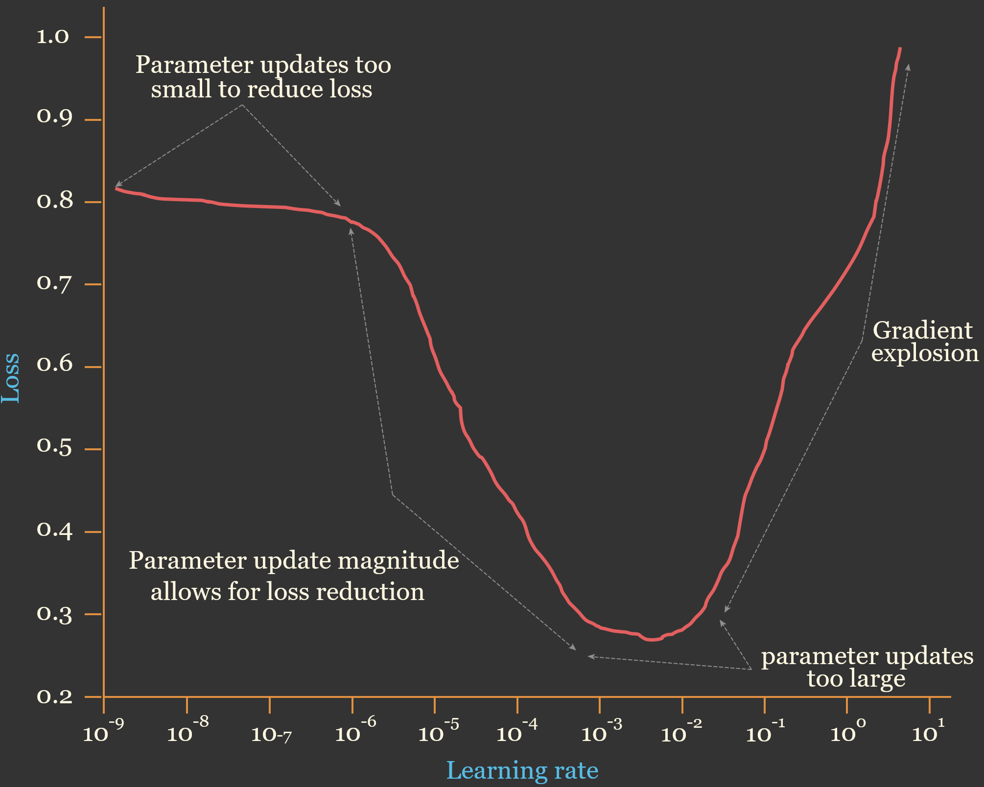
To learn more about how this process works, please consult the paper referenced above and/or the associated lecture module. Generally, the learning rate starts at a very low rate and is gradually increased to a larger rate. Initially, the loss will not decrease because the learning rate is too low to allow for meaningful parameter updates. As the learning rates increases, the loss should begin to decrease. However, eventually the learning rates will get too high and result in unstable learning and gradient explosion. The range of learning rates that are allowing for meaningful parameter updates, as estimated by reduction in the loss metric, without unstable learning or a gradient explosion, are suggested to be optimal. This process is conceptualized in Figure 7.5.

Figure 7.5. Conceptualization of the learning rate finder. At very low learning rates, the parameter updates are too small to reduce the loss. As the learning rate increases, the updates become large enough to reduce the loss. At high learning rates, the updates become too large, and the loss increases rapidly due to unstable learning and gradient explosion.

#!pip install torch-lr-finder

from torch_lr_finder import LRFinder

class myFCNLeaky(nn.Module):
  def __init__(self, inSize, hiddenSizes, outSize):
    super().__init__()
    self.inSize = inSize
    self.hiddenSize = hiddenSizes
    self.outSize = outSize

    self.theNetwork = nn.Sequential(
        nn.Linear(inSize, hiddenSizes[0]),
        nn.BatchNorm1d(hiddenSizes[0]),
        nn.LeakyReLU(negative_slope=0.1, inplace=True),
        nn.Linear(hiddenSizes[0], hiddenSizes[1]),
        nn.BatchNorm1d(hiddenSizes[1]),
        nn.LeakyReLU(negative_slope=0.1, inplace=True),
        nn.Linear(hiddenSizes[1], outSize)
    )

  def forward(self, x):
    x = self.theNetwork(x)
    return x

model = myFCNLeaky(10, [256, 256], 10).to(device)

Since the learning rate range test trains the model for 100 iterations, it is not executed here; the resulting plot is shown below.

criterion = nn.CrossEntropyLoss()
optimizer = torch.optim.AdamW(model.parameters())
lr_finder = LRFinder(model, optimizer, criterion, device="cuda")
lr_finder.range_test(trainDL, val_loader=valDL, start_lr=0.0001, end_lr=1, num_iter=100, step_mode="linear")
lr_finder.plot(log_lr=False)
lr_finder.reset()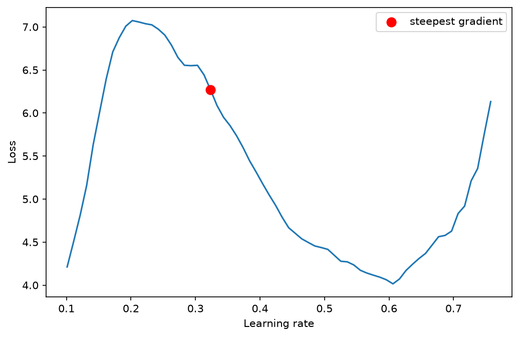

Loss versus learning rate from the learning rate range test. The red point marks the learning rate with the steepest negative slope.

7.10 Learning Rate Scheduling

Another technique that has proved to be useful is augmenting the learning rate throughout the training process. There are lots of different ways to do this. One of the simplest is to use a larger learning rate early in the training then reduce the learning rate after a defined number of epochs. The idea here is that the model can be more coarsely trained initially then fine-tuned with a lower learning rate during later epochs.

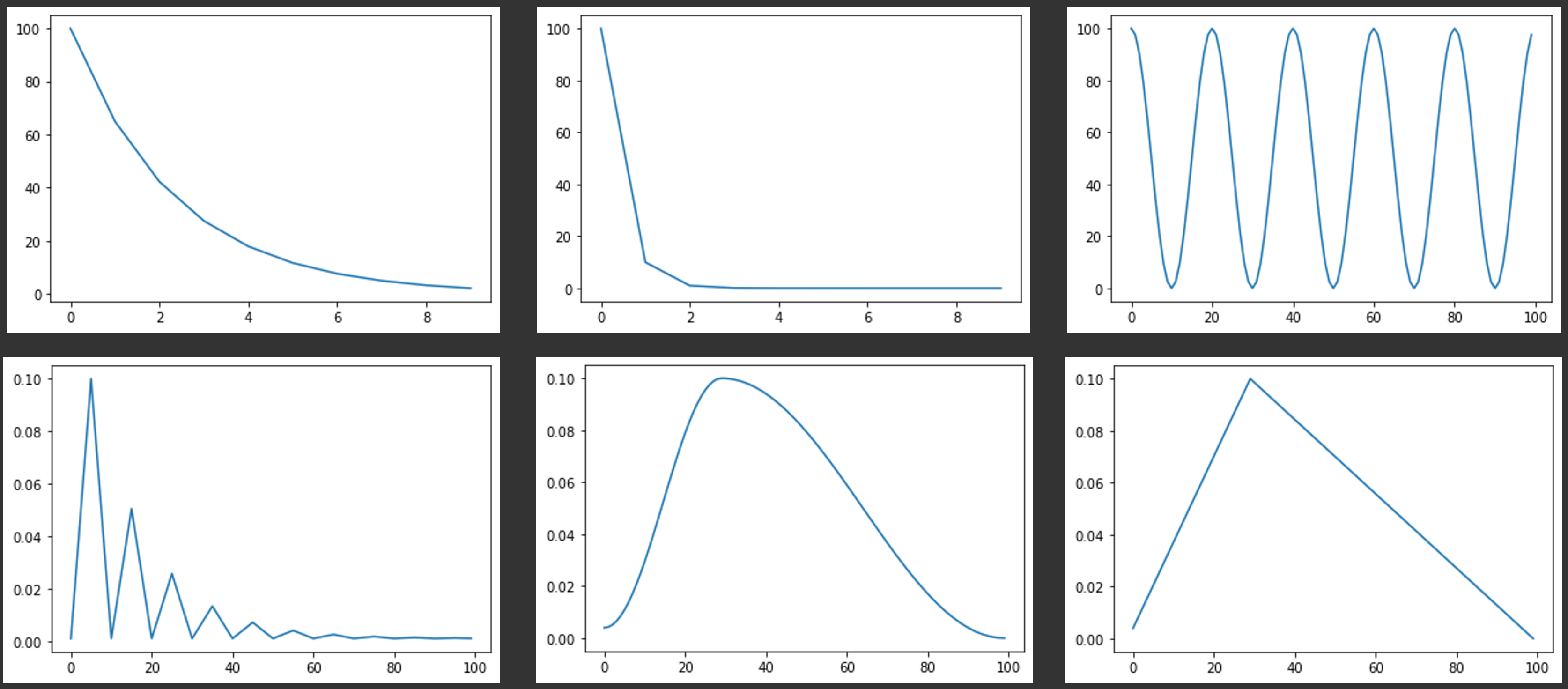
One method that has been shown to be especially effective is to implement a one cycle learning rate policy in which the learning rate starts low, raises to a maximum learning rate, then descends back to a low learning rate as a single cycle during the training process. This method was proposed by Leslie Smith in the same paper referenced above. This method has been implemented in PyTorch as a scheduler. Schedulers allow for modifying the training loop in some way by calling a step. Note that a variety of schedulers are available for different use cases. If you are interested in learning more about schedulers, please consult the PyTorch documentation.

To implement a one cycle learning rate in PyTorch, you can use the OneCycleLR() function. This allows for specifying the maximum learning rate, number of epochs, and number of steps per epoch (i.e., mini-batches). This information allows the algorithm to determine how to alter the learning rate over the entire learning process.

To actually augment the learning rate using this scheduler, you must call scheduler.step() in the training loop. Since this needs to happen after processing each mini-batch, this should be done within the mini-batch for loop for the training mini-batches. In the example below, I have called it after optimizer.step(). So, this is actually pretty easy to implement. It only requires (1) defining and instantiating an instance of the scheduler and (2) performing a step within each training mini-batch iteration in the training loop.

There are many other methods for augmenting learning rates. I recommend this post on Kaggle that demonstrates a variety of learning rate schedulers using PyTorch: https://www.kaggle.com/code/isbhargav/guide-to-pytorch-learning-rate-scheduling. Several of these schedulers are visualized in Figure 7.6.

Figure 7.6. Examples of learning rate schedulers, showing the learning rate (y-axis) at each epoch or iteration (x-axis). Top row: exponential decay with a slower (left) and faster (center) decay rate, and cosine annealing, in which the learning rate repeatedly decreases and increases following a cosine curve (right). Bottom row: a cyclical learning rate in which the maximum learning rate is halved with each cycle (left), and a one cycle policy with cosine (center) and linear (right) annealing.

optimizer = torch.optim.SGD(model.parameters(), lr=0.1, momentum=0.9)

scheduler = torch.optim.lr_scheduler.OneCycleLR(optimizer, max_lr=0.1, epochs=50, steps_per_epoch=len(trainDL))

criterion = nn.CrossEntropyLoss().to(device)

#Define assessment metrics
acc = tm.Accuracy(task="multiclass", num_classes=10).to(device)
f1 = tm.F1Score(task="multiclass", num_classes=10).to(device)
kappa = tm.CohenKappa(task="multiclass", num_classes=10).to(device)

epochs = 50

saveFolder = "data/output/"

eNum = []
t_loss = []
t_acc = []
t_f1 = []
t_kappa = []
v_loss = []
v_acc = []
v_f1 = []
v_kappa = []

#Loop over epochs
for epoch in range(1, epochs+1):
    #Put model in training mode
    model.train()
    #initialize running training loss
    running_loss = 0.0
    #Loop over batches
    for batch_idx, (inputs, targets) in enumerate(trainDL):
        #Get data and move to device
        inputs, targets = inputs.to(device), targets.to(device)

        #Clear gradients
        optimizer.zero_grad()
        #Predict data
        outputs = model(inputs)
        #Calculate loss
        loss = criterion(outputs, targets)

        #Update running with batch results
        running_loss += loss.item()

        #Calculate metrics
        accT = acc(outputs, targets)
        f1T = f1(outputs, targets)
        kappaT = kappa(outputs, targets)

        #Backpropagate
        loss.backward()

        # update parameters
        optimizer.step()
        scheduler.step()

    # Accumulate loss and metrics at end of training epoch
    epoch_loss = running_loss/len(trainDL)
    accT = acc.compute()
    f1T = f1.compute()
    kappaT = kappa.compute()

    # Print Losses and metrics at end of each Epoch
    print(f'Epoch: {epoch}, Training Loss: {epoch_loss:.4f}, Training Accuracy: {accT:.4f}, Training F1: {f1T:.4f}, Training Kappa: {kappaT:.4f}')

     #Append results
    eNum.append(epoch_loss)
    t_loss.append(loss.item())
    t_acc.append(accT.detach().cpu().numpy())
    t_f1.append(f1T.detach().cpu().numpy())
    t_kappa.append(kappaT.detach().cpu().numpy())

    #Reset metrics
    acc.reset()
    f1.reset()
    kappa.reset()

    #Set model in evaluation model
    model.eval()
    # loop over validation batches
    with torch.no_grad():
        for batch_idx, (inputs, targets) in enumerate(valDL):
            #Get data and move to device
            inputs, targets = inputs.to(device), targets.to(device)

            #Predict data
            outputs = model(inputs)
            #Calculate validation loss
            loss_v = criterion(outputs, targets)

            #Update running with batch results
            running_loss_v += loss_v.item()

            #Accumulate loss and metrics at end of validation epoch
            epoch_loss_v = running_loss_v/len(valDL)
            accV = acc(outputs, targets)
            f1V = f1(outputs, targets)
            kappaV = kappa(outputs, targets)

    #Accumulate metrics at end of epoch
    accV = acc.compute()
    f1V = f1.compute()
    kappaV = kappa.compute()

    #Print validation loss and metrics
    print(f'Validation Loss: {epoch_loss_v:.4f}, Validation Accuracy: {accV:.4f}, Validation F1: {f1V:.4f}, Validation Kappa: {kappaV:.4f}')

    #Append results
    v_loss.append(epoch_loss_v)
    v_acc.append(accV.detach().cpu().numpy())
    v_f1.append(f1V.detach().cpu().numpy())
    v_kappa.append(kappaV.detach().cpu().numpy())

    #Reset metrics
    acc.reset()
    f1.reset()
    kappa.reset()

    torch.save(model.state_dict(), saveFolder + 'eurosat_model_' + str(epoch) + '.pt')
    print(f'Model saved for epoch {epoch}.')

7.11 Gradient Accumulation

Very small mini-batch sizes can result in noisy or suboptimal parameter updates. However, it is not always possible to use a large mini-batch size. For example, if you are using large image chips, a complex architecture, and/or have limited GPU VRAM, you may not be able to use a large mini-batch size. To get around this issue, you can implement gradient accumulation. The idea here is that the weights/parameters are not updated after each training mini-batch is processed. Instead, the gradients are allowed to accumulate over a given number of mini-batches prior to performing the optimization.

In the example below, I am allowing the gradients to accumulate for 4 mini-batches before applying the optimization or weight/parameter updates. This involves (1) defining a variable, in this case accum_iter, that specifies over how many mini-batches to accumulate the losses, (2) dividing the loss by this variable for normalization, (3) defining a condition with an if statement so that gradients will only be updated after every 4 mini-batches or for the final training mini-batch, and (5) only applying the optimizer and clearing the gradients if one of these conditions are met. In my example below, this condition is applied inside of the for loop that iterates over the mini-batches and after the loss has been calculated and the backpropagation has been performed. Also, I am not clearing the gradients at the beginning of each training mini-batch. Instead, this occurs within the conditions since accumulating the gradients cannot occur if they are cleared. So, the gradients are only cleared after an optimization step has been performed.

In this specific example, gradient accumulation is not necessary since the mini-batch size is large. This is just an example. Also, large mini-batch sizes can be problematic. So, use gradient accumulation with care.

eNum = []
t_loss = []
t_acc = []
t_f1 = []
t_kappa = []
v_loss = []
v_acc = []
v_f1 = []
v_kappa = []

#Loop over epochs
for epoch in range(1, epochs+1):
    #Put model in training mode
    model.train()
    #initialize running training loss
    running_loss = 0.0
    #Loop over batches
    for batch_idx, (inputs, targets) in enumerate(trainDL):
        #Get data and move to device
        inputs, targets = inputs.to(device), targets.to(device)

        #Clear gradients
        optimizer.zero_grad()
        #Predict data
        outputs = model(inputs)
        #Calculate loss
        loss = criterion(outputs, targets)

        #Update running with batch results
        running_loss += loss.item()

        #Calculate metrics
        accT = acc(outputs, targets)
        f1T = f1(outputs, targets)
        kappaT = kappa(outputs, targets)

        #Backpropagate
        loss.backward()

        # Implement gradient accumulation
        if ((batch_idx + 1) % accum_iter == 0) or (batch_idx + 1 == len(trainDL)):
            optimizer.step()
            optimizer.zero_grad()

    # Accumulate loss and metrics at end of training epoch
    epoch_loss = running_loss/len(trainDL)
    accT = acc.compute()
    f1T = f1.compute()
    kappaT = kappa.compute()

    # Print Losses and metrics at end of each Epoch
    print(f'Epoch: {epoch}, Training Loss: {epoch_loss:.4f}, Training Accuracy: {accT:.4f}, Training F1: {f1T:.4f}, Training Kappa: {kappaT:.4f}')

     #Append results
    eNum.append(epoch_loss)
    t_loss.append(loss.item())
    t_acc.append(accT.detach().cpu().numpy())
    t_f1.append(f1T.detach().cpu().numpy())
    t_kappa.append(kappaT.detach().cpu().numpy())

    #Reset metrics
    acc.reset()
    f1.reset()
    kappa.reset()

    #Set model in evaluation model
    model.eval()
    # loop over validation batches
    with torch.no_grad():
        for batch_idx, (inputs, targets) in enumerate(valDL):
            #Get data and move to device
            inputs, targets = inputs.to(device), targets.to(device)

            #Predict data
            outputs = model(inputs)
            #Calculate validation loss
            loss_v = criterion(outputs, targets)

            #Update running with batch results
            running_loss_v += loss_v.item()

            #Accumulate loss and metrics at end of validation epoch
            epoch_loss_v = running_loss_v/len(valDL)
            accV = acc(outputs, targets)
            f1V = f1(outputs, targets)
            kappaV = kappa(outputs, targets)

    #Accumulate metrics at end of epoch
    accV = acc.compute()
    f1V = f1.compute()
    kappaV = kappa.compute()

    #Print validation loss and metrics
    print(f'Validation Loss: {epoch_loss_v:.4f}, Validation Accuracy: {accV:.4f}, Validation F1: {f1V:.4f}, Validation Kappa: {kappaV:.4f}')

    #Append results
    v_loss.append(epoch_loss_v)
    v_acc.append(accV.detach().cpu().numpy())
    v_f1.append(f1V.detach().cpu().numpy())
    v_kappa.append(kappaV.detach().cpu().numpy())

    #Reset metrics
    acc.reset()
    f1.reset()
    kappa.reset()

    torch.save(model.state_dict(), saveFolder + 'eurosat_model_' + str(epoch) + '.pt')
    print(f'Model saved for epoch {epoch}.')

7.12 Using Multiple GPUs

Training on multiple GPUs is an effective means to speed up the training process. So, if you are fortunate enough to have access to a computer with multiple CUDA-enabled GPUs or a GPU cluster, I highly recommend augmenting your code to make use of this hardware. The code below shows how to get the count of available GPUs.

devCnt = torch.cuda.device_count()

There are a few methods that can be used to train your model over multiple GPUs. I tend to use nn.DataParallel(). This allows for partitioning the training mini-batches into multiple smaller mini-batches that are then processed on separate GPUs in parallel.

Implementing this method is very easy. You simply need to wrap your model in this function, as demonstrated below, then move it to the device. The training loop can then be implemented as normal.

model = nn.DataParallel(model)

model.to(DEVICE)

model.module.load_state_dict("PATH TO SAVED PARAMETERS")

7.13 Enhancing Reproducibility

Lastly, you may want to be able to obtain the same results when running the training process multiple times. Obtaining reproducibility is complex with PyTorch, especially when using GPU-based computation. The following paper provides some guidance on obtaining reproducibility within PyTorch:

Alahmari, S.S., Goldgof, D.B., Mouton, P.R. and Hall, L.O., 2020. “Challenges for the repeatability of deep learning models.” IEEE Access, 8, pp.211860-211868.

Randomness enters the training process in many places, including the initialization of the model parameters, the shuffling of the training data, random data augmentations, dropouts, and random sampling of the data partitions. Each of these is controlled by a random number generator. Python, NumPy, and PyTorch each have their own generators, and PyTorch maintains separate generators for the CPU and each GPU. In addition, some GPU operations are non-deterministic: they can return slightly different results each time they are run, even with the same inputs, because the order in which values are summed in parallel can vary, and floating-point addition is not perfectly associative. These small differences can grow over many training iterations.

The function below sets all of the random seeds and configures PyTorch to use deterministic algorithms:

1. random.seed(), np.random.seed(), and torch.manual_seed() seed the Python, NumPy, and PyTorch generators. torch.manual_seed() also seeds the generators for all GPUs, and torch.cuda.manual_seed_all() is included to make this explicit.
2. torch.backends.cudnn.deterministic = True forces the cuDNN library, which implements many GPU operations, such as convolution, to use deterministic algorithms, and torch.backends.cudnn.benchmark = False stops cuDNN from benchmarking and selecting the fastest algorithm for your hardware, since the selected algorithm can vary between runs.
3. torch.use_deterministic_algorithms(True) goes further and requires all PyTorch operations to use deterministic implementations. If an operation does not have a deterministic implementation, an error is raised so that you know reproducibility cannot be guaranteed. Setting warn_only=True issues a warning as opposed to an error. Some operations, such as the backward pass of bilinear upsampling on the GPU, which is common in semantic segmentation architectures, do not have deterministic implementations, so warn_only=True may be necessary.
4. The CUBLAS_WORKSPACE_CONFIG environment variable must be set for some GPU matrix operations to be deterministic. It must be set before these operations are first used, so it is best to set it at the very beginning of your script.

import os
os.environ["CUBLAS_WORKSPACE_CONFIG"] = ":4096:8"  # set before any CUDA operations

def set_seed(seed=42, deterministic=True, warn_only=True):
    random.seed(seed)
    np.random.seed(seed)
    torch.manual_seed(seed)
    torch.cuda.manual_seed_all(seed)
    if deterministic:
        torch.backends.cudnn.deterministic = True
        torch.backends.cudnn.benchmark = False
        torch.use_deterministic_algorithms(True, warn_only=warn_only)

set_seed(42)

Setting the seeds is not enough when the DataLoader uses multiple worker processes (num_workers > 0), since each worker has its own random state, which affects random augmentations applied in the DataSet. The shuffling order is also determined by a generator. To make data loading reproducible, a worker_init_fn that seeds each worker and a seeded torch.Generator should be passed to the DataLoader.

def seed_worker(worker_id):
    worker_seed = torch.initial_seed() % 2**32
    np.random.seed(worker_seed)
    random.seed(worker_seed)

g = torch.Generator()
g.manual_seed(42)

trainDL = DataLoader(trainDS, batch_size=256, shuffle=True, drop_last=True,
                     num_workers=4, worker_init_fn=seed_worker, generator=g)

So, is this enough to make the training process fully reproducible? With all of these settings, repeated runs on the same machine, with the same hardware, drivers, and package versions, should produce the same results, or very nearly the same results if some operations were allowed to run non-deterministically using warn_only=True. However, there are some important limitations:

1. Results are not guaranteed to be identical across different GPUs, CPU versus GPU computation, different versions of PyTorch, CUDA, or cuDNN, or different operating systems.
2. Some operations do not have deterministic implementations. If you require exact reproducibility, you must avoid these operations or run them on the CPU.
3. Deterministic algorithms can be slower than their non-deterministic counterparts, so training time may increase.
4. Training on multiple GPUs introduces additional sources of non-determinism.

In practice, I recommend setting the seeds and the deterministic settings while developing and debugging a workflow, since being able to reproduce a result makes it much easier to determine whether a change to the code had an impact. When comparing models, it is generally more informative to train each configuration several times with different seeds and compare the distributions of the results, since the variability between runs with different seeds can be as large as the difference between configurations. As you will see in Chapter 8, PyTorch Lightning simplifies this process with its seed_everything() function and the deterministic argument of its Trainer class.

7.14 Concluding Remarks

The goal of this chapter was to introduce some common methods that can be used to potentially improve the performance of the final model and/or to combat some common issues, such as class imbalance and overfitting. If you are struggling with your training process, it might be worth investigating these techniques. It is also a good idea to explore the internet, blogs, and help sites for other suggestions that might be appropriate for your specific use case. Also, deep learning techniques are still developing, so new methods may be proposed that are not presented here. With that said, I have found the methods that I discussed here to be especially useful.

You may have noticed that many of these modifications, such as learning rate scheduling, gradient accumulation, multi-GPU training, and reproducibility settings, required editing the training loop, and the training loop has become long and error-prone. In the next chapter, we will explore PyTorch Lightning, which handles the training loop for us and makes many of these modifications as simple as setting an argument. We will continue to discuss methods to improve models in later chapters, including transfer learning (Chapter 13) and architecture modifications (Chapter 18).

7.15 Questions

1. Explain how dropouts are implemented and why they may reduce overfitting. Why are dropouts now less commonly used?
2. What is the “dying ReLU” problem? Explain how the leaky ReLU, Swish, and GELU activation functions differ from ReLU and how each addresses this problem.
3. Explain how class weights are calculated using the inverse of the relative abundance of each class and how they are incorporated into the cross entropy loss calculation.
4. Explain how label smoothing modifies the target probabilities used by cross entropy loss. With a smoothing factor of 0.1 and 5 classes, what are the target probabilities for the correct class and each incorrect class? Why does label smoothing discourage overconfident predictions?
5. Explain how a WeightedRandomSampler() can be used to combat class imbalance. Why is this method more difficult to apply to semantic segmentation tasks than to scene labeling tasks?
6. Describe the one cycle learning rate policy. When using OneCycleLR(), where in the training loop must scheduler.step() be called, and why?
7. Explain the purpose of gradient accumulation and how the training loop must be modified to implement it.
8. List the steps required to make a PyTorch training process reproducible, including those related to the DataLoader. Why can exact reproducibility still not be guaranteed across different hardware or software versions?

7.16 Exercises

Exercise 7.1: ANN Model Comparisons

Introduction

This exercise expands upon Exercise 6.1 by asking you to compare models with different configurations or training routines. We recommend re-running your code from Exercise 6.1 and then continuing with the new analyses. You will work with the same Covertype dataset (covertype.csv in the data/files/tables folder), forest type classes, and predictor variables used in Exercise 6.1.

Deliverables

• A Quarto (.qmd) file containing all required code and answers to the questions and discussion prompts, and the HTML webpage rendered from it

Tasks

Models

Compare the results obtained in Exercise 6.1 with results obtained using the following modifications. Including the model from Exercise 6.1, you should train a total of five models. Make sure to log all training and validation losses by epoch. Train all models for 50 epochs using the same training and validation data.

Task 1: Replace the ReLU layers with leaky ReLU and re-train the model.

Task 2: Re-train the model from Exercise 6.1 using the AdamW optimizer as opposed to stochastic gradient descent. Use a learning rate of 0.001.

Task 3: Re-train the model from Exercise 6.1 using cross entropy loss with class weights. Weights should be scaled relative to the inverse of the abundance of each class in the training dataset.

Task 4: Implement a one cycle learning rate policy where the learning rate increases from a base learning rate of 0.0001 to a maximum learning rate of 0.1 and then decreases back to 0.0001 over the entire training process.

Comparisons

Task 5: Create a plot of training losses across all 50 epochs for all five experiments.

Task 6: Create a plot of validation losses across all 50 epochs for all five experiments.

Task 7: Using torchmetrics and the test data, calculate overall accuracy and class-aggregated, macro-averaged precision, recall, and F1-score for each model.

Task 8: Discuss your results. Did any of the four tested alterations improve the model’s performance? How do the loss curves and the assessment metrics calculated from the withheld test data compare between the models?