import numpy as np
import pandas as pd
import matplotlib.pyplot as plt
import rasterio as rio

import torch
import torch.nn as nn
import torch.nn.functional as F
from torch.utils.data import Dataset, DataLoader
import lightning as L
from lightning.pytorch.callbacks import ModelCheckpoint, LearningRateMonitor, BaseFinetuning
from lightning.pytorch.loggers import CSVLogger
from torchinfo import summary27 Pre-Training with Fully Convolutional Masked Autoencoders
27.1 Introduction
Throughout this text, we have trained models using supervised learning, in which every training sample has a label. In Chapter 13 and Chapter 17, we initialized models using parameters learned from ImageNet, a large labeled dataset of photographs. However, labeled geospatial data are expensive to produce, since they generally require manual interpretation or field work, and ImageNet photographs are very different from multispectral satellite imagery, aerial orthophotography, or digital terrain data. At the same time, enormous amounts of unlabeled geospatial data are freely available, such as the Landsat and Sentinel-2 archives and national lidar collections.
Self-supervised learning (SSL) makes it possible to learn potentially useful representations from unlabeled data. The model is trained to solve a pretext task for which the labels are derived from the data themselves. The pre-trained encoder is then fine-tuned for the task of interest, the downstream task, using a smaller labeled dataset. Two major families of SSL methods are:
- Contrastive and self-distillation methods, such as SimCLR, MoCo, and DINO, which train the model to produce similar representations for different augmented views of the same image.
- Masked image modeling, in which a portion of the input is hidden and the model is trained to reconstruct it. The most influential example is the masked autoencoder (MAE) (He et al., 2022), which hides a large proportion (75%) of the image patches input to a Vision Transformer and trains the model to reconstruct the missing pixels. To succeed, the model must learn the structure of the data, such as the shapes, textures, and spatial arrangements of land surface features.
He, K., Chen, X., Xie, S., Li, Y., Dollár, P. and Girshick, R., 2022. “Masked autoencoders are scalable vision learners.” In Proceedings of the IEEE/CVF Conference on Computer Vision and Pattern Recognition (pp. 16000-16009).
The MAE was designed for transformers, which operate on sequences of patches, so the masked patches can simply be removed from the sequence. Applying the same idea to CNNs is more difficult. A convolution slides over the entire image, so (1) the encoder must process the masked regions, which wastes computation, and (2) information can leak into the masked regions from their visible neighbors as the kernels pass over the boundaries between masked and visible areas, making the task easier than intended and changing the statistics of the features. The fully convolutional masked autoencoder (FCMAE), introduced with ConvNeXt V2 (Woo et al., 2023), solves this problem by treating the visible portion of the image as a sparse input, as if the masked pixels did not exist.
Woo, S., Debnath, S., Hu, R., Chen, X., Liu, Z., Kweon, I.S. and Xie, S., 2023. “ConvNeXt V2: Co-designing and scaling ConvNets with masked autoencoders.” In Proceedings of the IEEE/CVF Conference on Computer Vision and Pattern Recognition (pp. 16133-16142).
The FCMAE architecture is conceptualized in Figure 27.1. A large proportion of the input image is randomly masked. The encoder, a ConvNeXt V2 model, consists of a stem that reduces the spatial dimensions by a factor of 4 followed by four stages of blocks, which further reduce the spatial dimensions to 1/32 of the input. A lightweight decoder and a prediction head generate predictions for each patch, which are rearranged, or unpatchified, back into an image with the original spatial dimensions. The loss is calculated using only the masked regions, so the model must predict the hidden content from the visible content. After pre-training, the decoder and prediction head are discarded, and the encoder is used for the downstream task.
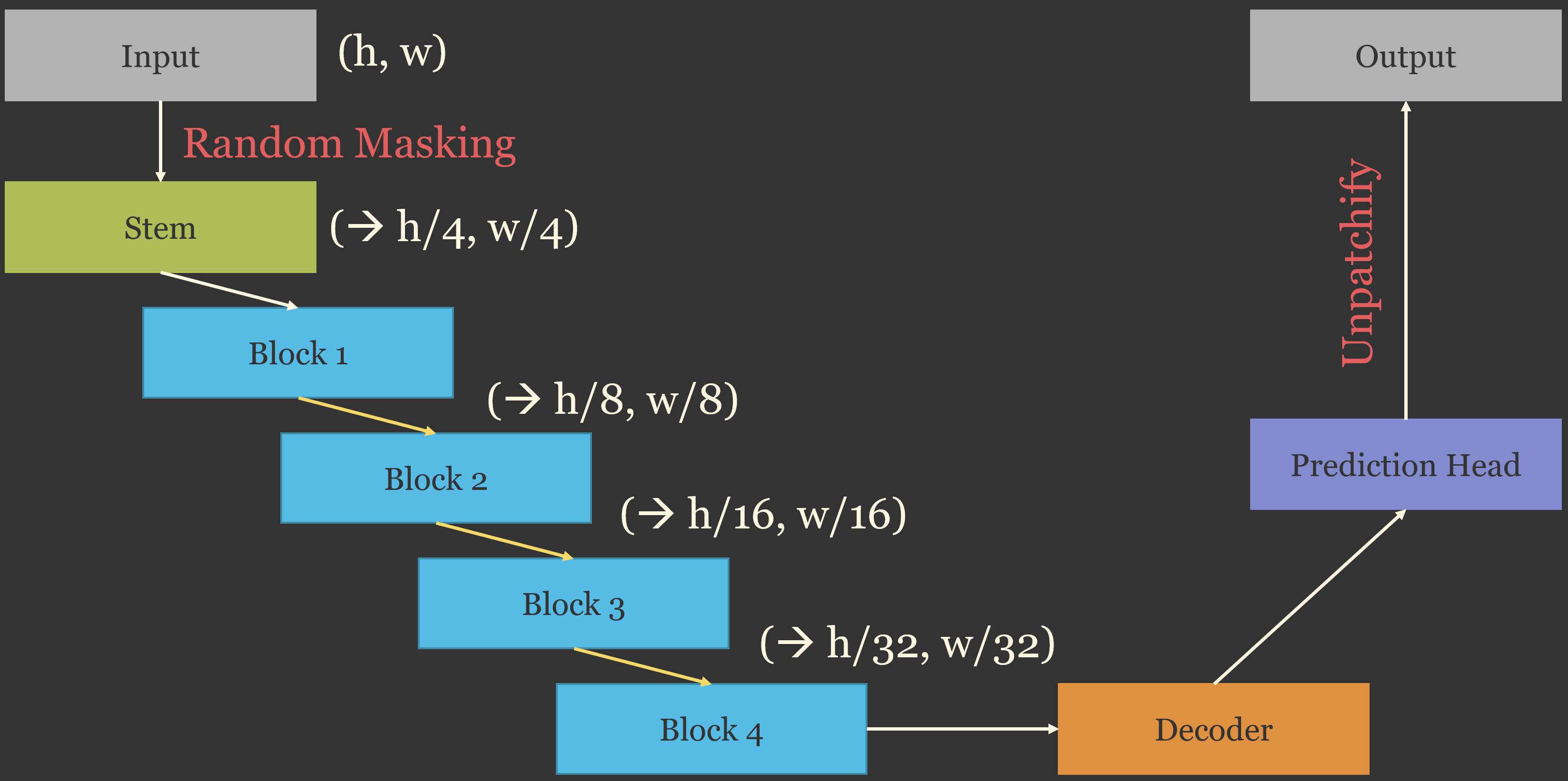
In this chapter, I explain and build the FCMAE, demonstrate how to pre-train it on unlabeled image chips using PyTorch Lightning, and show how to use the pre-trained encoder in a UNet-like architecture for semantic segmentation. The example uses the vfillDLMini dataset, a subset of the vfillDL valley fill face dataset introduced in Chapter 20. Each chip is a three-band stack of land surface parameters (LSPs) derived from a lidar digital terrain model, and the FCMAE is trained to reconstruct this stack. This chapter builds on the ConvNeXt and ConvNeXt V2 architectures discussed in Chapter 24.
27.2 The FCMAE Design
The FCMAE consists of the following components:
- Masking: the image is divided into square patches whose size equals the total downsampling factor of the encoder (32x32 pixels for ConvNeXt), and a random 60% of the patches are masked. The masking ratio is lower than the 75% used by the MAE, since the hierarchical CNN encoder benefits from more visible context.
- Encoder: a ConvNeXt V2 encoder processes only the visible patches. In the original implementation, this is accomplished using sparse convolution, which only computes outputs at visible locations. An equivalent, simpler approach for experimentation is dense masking: the masked regions are set to zero at the input and after every block, so that no information flows from visible to masked regions. Dense masking produces the same results as sparse convolution for the visible locations but does not save computation. I use dense masking here since it does not require a sparse convolution library. The global response normalization (GRN) layer introduced in Chapter 24 was designed specifically to prevent feature collapse during FCMAE pre-training.
- Decoder: a deliberately lightweight decoder, consisting of a single ConvNeXt block, operates at the lowest resolution (1/32 of the input). The encoder’s output at the masked locations is replaced with a learnable mask token, and the decoder predicts the pixel values of each 32x32 patch from the corresponding location in the 1/32-resolution feature maps. Keeping the decoder small forces the encoder to learn the useful representations, since the encoder, not the decoder, is kept for the downstream task.
- Loss: the mean squared error between the predicted and actual pixel values, calculated only for the masked patches. The model is not rewarded for reproducing the visible pixels, which it could do trivially. As in the MAE, the target pixels within each patch are normalized using that patch’s mean and variance, which encourages the model to focus on local structure as opposed to overall brightness.
27.3 Building the FCMAE
27.3.1 Patches and Masks
I begin by defining functions to convert images to patches and back and to generate random masks. The patchify() function converts a tensor with a shape of (N, C, H, W) into a tensor with a shape of (N, L, P×P×C), where L is the number of patches and P is the patch size, so that each row contains all of the values in one patch. The randomMask() function generates a binary mask with a shape of (N, H/P, W/P), in which 1 indicates a masked patch and 0 indicates a visible patch. Exactly the requested proportion of patches is masked in each image.
def patchify(imgs, p):
    N, C, H, W = imgs.shape
    h, w = H // p, W // p
    x = imgs.reshape(N, C, h, p, w, p)
    x = torch.einsum("nchpwq->nhwpqc", x)
    return x.reshape(N, h * w, p * p * C)

def unpatchify(x, p, C, h, w):
    N = x.shape[0]
    x = x.reshape(N, h, w, p, p, C)
    x = torch.einsum("nhwpqc->nchpwq", x)
    return x.reshape(N, C, h * p, w * p)

def randomMask(N, h, w, ratio, device):
    L = h * w
    nMask = int(round(L * ratio))
    noise = torch.rand(N, L, device=device)
    ids = torch.argsort(noise, dim=1)                 # random permutation per image
    mask = torch.zeros(N, L, device=device)
    mask.scatter_(1, ids[:, :nMask], 1.0)             # first nMask positions are masked
    return mask.reshape(N, h, w)
27.3.2 Masked ConvNeXt V2 Encoder
The encoder follows the ConvNeXt V2 design: a patchify stem (a 4x4 convolution with a stride of 4 followed by layer normalization), four stages of ConvNeXt V2 blocks, and downsampling layers between the stages (layer normalization followed by a 2x2 convolution with a stride of 2). The LayerNorm2d and ConvNeXtV2Block classes were defined in Chapter 24 and are repeated here.
The forward() method accepts an optional mask. If a mask is provided, it is upsampled to the resolution of each stage using nearest neighbor interpolation, and the feature maps are multiplied by the inverted mask (1 for visible, 0 for masked) after the stem and after every block, which implements dense masking. If no mask is provided, which is the case when the encoder is used for the downstream task, the encoder behaves as a standard ConvNeXt V2. The method returns the feature maps from all four stages, which will be needed by the segmentation decoder.
class LayerNorm2d(nn.Module):
    def __init__(self, nChn, eps=1e-6):
        super().__init__()
        self.weight = nn.Parameter(torch.ones(nChn))
        self.bias = nn.Parameter(torch.zeros(nChn))
        self.eps = eps

    def forward(self, x):
        mean = x.mean(1, keepdim=True)
        var = (x - mean).pow(2).mean(1, keepdim=True)
        x = (x - mean) / torch.sqrt(var + self.eps)
        return x * self.weight[:, None, None] + self.bias[:, None, None]

class GRN(nn.Module):
    def __init__(self, dim):
        super().__init__()
        self.gamma = nn.Parameter(torch.zeros(1, 1, 1, dim))
        self.beta = nn.Parameter(torch.zeros(1, 1, 1, dim))

    def forward(self, x):
        gx = torch.norm(x, p=2, dim=(1, 2), keepdim=True)
        nx = gx / (gx.mean(dim=-1, keepdim=True) + 1e-6)
        return self.gamma * (x * nx) + self.beta + x

class ConvNeXtV2Block(nn.Module):
    def __init__(self, dim, mlpRatio=4):
        super().__init__()
        self.dwconv = nn.Conv2d(dim, dim, kernel_size=7, padding=3, groups=dim)
        self.norm = nn.LayerNorm(dim, eps=1e-6)
        self.pwconv1 = nn.Linear(dim, mlpRatio * dim)
        self.act = nn.GELU()
        self.grn = GRN(mlpRatio * dim)
        self.pwconv2 = nn.Linear(mlpRatio * dim, dim)

    def forward(self, x):
        y = self.dwconv(x).permute(0, 2, 3, 1)
        y = self.pwconv2(self.grn(self.act(self.pwconv1(self.norm(y))))).permute(0, 3, 1, 2)
        return x + y

class MaskedConvNeXtV2Encoder(nn.Module):
    def __init__(self, inChn=3, dims=(96, 192, 384, 768), depths=(2, 2, 6, 2)):
        super().__init__()
        self.dims = dims
        self.stem = nn.Sequential(nn.Conv2d(inChn, dims[0], kernel_size=4, stride=4), LayerNorm2d(dims[0]))
        self.downs = nn.ModuleList([nn.Sequential(LayerNorm2d(dims[i]),
                                                  nn.Conv2d(dims[i], dims[i + 1], kernel_size=2, stride=2))
                                    for i in range(3)])
        self.stages = nn.ModuleList([nn.ModuleList([ConvNeXtV2Block(dims[i]) for _ in range(depths[i])])
                                     for i in range(4)])

    def forward(self, x, mask=None):
        keep = None
        x = self.stem(x)
        feats = []
        for i in range(4):
            if i > 0:
                x = self.downs[i - 1](x)
            if mask is not None:
                keep = 1.0 - F.interpolate(mask.unsqueeze(1), size=x.shape[2:], mode="nearest")
                x = x * keep
            for blk in self.stages[i]:
                x = blk(x)
                if keep is not None:
                    x = x * keep          # dense masking: no information enters masked regions
            feats.append(x)
        return feats                       # resolutions 1/4, 1/8, 1/16, 1/32
The default settings correspond approximately to the Tiny version of ConvNeXt V2 with fewer blocks in the third stage, which reduces the computation required for pre-training. The dims and depths arguments can be changed to create smaller or larger encoders.
27.3.3 Decoder and Complete Model
The FCMAE class combines the encoder and decoder and calculates the loss. In the forward() method:
- A random mask is generated at the patch resolution (1/32 of the input).
- The masked image is passed through the encoder, and the output of the last stage is projected to the decoder width using a 1x1 convolution.
- At the masked locations, the projected features are replaced with the learnable mask token, which is broadcast to every masked location.
- A single ConvNeXt V2 block processes the result, and a 1x1 convolution predicts P×P×C values (the pixels of one patch) at each location.
- The loss is calculated as the mean squared error between the predicted and normalized target pixels, averaged over the pixels in each patch and then over the masked patches only.
class FCMAE(nn.Module):
    def __init__(self, inChn=3, dims=(96, 192, 384, 768), depths=(2, 2, 6, 2),
                 decDim=512, maskRatio=0.6, patchSize=32, normPixLoss=True):
        super().__init__()
        self.inChn = inChn
        self.p = patchSize
        self.maskRatio = maskRatio
        self.normPixLoss = normPixLoss
        self.encoder = MaskedConvNeXtV2Encoder(inChn, dims, depths)
        self.proj = nn.Conv2d(dims[-1], decDim, kernel_size=1)
        self.maskToken = nn.Parameter(torch.zeros(1, decDim, 1, 1))
        self.decoder = ConvNeXtV2Block(decDim)
        self.pred = nn.Conv2d(decDim, patchSize * patchSize * inChn, kernel_size=1)

    def forward(self, imgs):
        N, C, H, W = imgs.shape
        h, w = H // self.p, W // self.p
        mask = randomMask(N, h, w, self.maskRatio, imgs.device)          # (N, h, w), 1 = masked

        x = self.encoder(imgs, mask)[-1]                                 # (N, dims[-1], h, w)
        x = self.proj(x)
        m = mask.unsqueeze(1)
        x = x * (1 - m) + self.maskToken * m                             # fill masked locations
        pred = self.pred(self.decoder(x))                                # (N, p*p*C, h, w)
        pred = pred.flatten(2).transpose(1, 2)                           # (N, L, p*p*C)

        target = patchify(imgs, self.p)                                  # (N, L, p*p*C)
        if self.normPixLoss:
            mean = target.mean(dim=-1, keepdim=True)
            var = target.var(dim=-1, keepdim=True)
            target = (target - mean) / (var + 1e-6) ** 0.5

        lossPerPatch = ((pred - target) ** 2).mean(dim=-1)              # (N, L)
        maskFlat = mask.flatten(1)
        loss = (lossPerPatch * maskFlat).sum() / maskFlat.sum()          # masked patches only
        return loss, pred, mask
To check the model, I pass a random tensor with the same shape as the vfillDLMini chips (three bands and 512x512 cells). Since each chip contains 16x16 = 256 patches of 32x32 cells, the predictions have a shape of (N, 256, 32×32×3) and the mask has a shape of (N, 16, 16).
model = FCMAE(inChn=3)
x = torch.rand(2, 3, 512, 512)
loss, pred, mask = model(x)
print(loss.item(), pred.shape, mask.shape)   # pred: (2, 256, 3072); mask: (2, 16, 16)
1.0124835968017578 torch.Size([2, 256, 3072]) torch.Size([2, 16, 16])summary(model.encoder, (2, 3, 512, 512), depth=2)==========================================================================================
Layer (type:depth-idx) Output Shape Param #
==========================================================================================
MaskedConvNeXtV2Encoder [2, 96, 128, 128] --
├─Sequential: 1-1 [2, 96, 128, 128] --
│ └─Conv2d: 2-1 [2, 96, 128, 128] 4,704
│ └─LayerNorm2d: 2-2 [2, 96, 128, 128] 192
├─ModuleList: 1-8 -- (recursive)
│ └─ModuleList: 2-3 -- 159,936
├─ModuleList: 1-7 -- (recursive)
│ └─Sequential: 2-4 [2, 192, 64, 64] 74,112
├─ModuleList: 1-8 -- (recursive)
│ └─ModuleList: 2-5 -- 614,784
├─ModuleList: 1-7 -- (recursive)
│ └─Sequential: 2-6 [2, 384, 32, 32] 295,680
├─ModuleList: 1-8 -- (recursive)
│ └─ModuleList: 2-7 -- 7,227,648
├─ModuleList: 1-7 -- (recursive)
│ └─Sequential: 2-8 [2, 768, 16, 16] 1,181,184
├─ModuleList: 1-8 -- (recursive)
│ └─ModuleList: 2-9 -- 9,537,024
==========================================================================================
Total params: 19,095,264
Trainable params: 19,095,264
Non-trainable params: 0
Total mult-adds (Units.GIGABYTES): 2.75
==========================================================================================
Input size (MB): 6.29
Forward/backward pass size (MB): 1431.31
Params size (MB): 76.38
Estimated Total Size (MB): 1513.98
==========================================================================================27.4 Pre-Training with Lightning
27.4.1 Unlabeled Data
The FCMAE requires only images. Any set of image chips can be used, including chips without labels and chips from areas or dates for which no reference data exist, which is the key advantage of self-supervised learning. Here, I use the image chips from the vfillDLMini training set and simply ignore the associated masks. The “trainDF.csv” file lists each chip’s file name (“chpN”) and whether it contains valley fill faces (“division”: “Positive” or “Background”). The chips are stored in subfolders named using the lowercase division, so I build the full path to each chip from these columns.
To keep the training time short, I pre-train using a random sample of 100 chips. In practice, pre-training should use as many unlabeled chips as possible, ideally many more than are available for the downstream task.
ImportantData Location
This chapter uses the vfillDLMini dataset, a subset of the vfillDL dataset, which is provided as a separate download (vfillDLMini.zip) in the download menu in the sidebar. By default, the code expects the uncompressed vfillDLMini folder to be saved in the data/files folder (data/files/vfillDLMini). If you saved the data elsewhere, set folder below to the folder’s location on your machine.
# Set this to the location of the uncompressed vfillDLMini folder on your machine.
folder = "data/files/vfillDLMini/"

trainDF = pd.read_csv(folder + "trainDF.csv")
trainDF["chpPth"] = folder + "train/images/" + trainDF["division"].str.lower() + "/" + trainDF["chpN"]
ssDF = trainDF.sample(n=100, random_state=42)
ssDF["division"].value_counts()
division
Positive 52
Background 48
Name: count, dtype: int64The DataSet below reads the chips from a list of file paths and applies light augmentations. Strong augmentations are generally unnecessary for masked image modeling since the masking itself makes the task difficult. The chip size must be divisible by the patch size (32), which is the case for these 512x512 chips. The three LSPs in each chip have already been rescaled to a range of 0 to 1, so no additional normalization is applied. Since the normalized-pixel loss normalizes each patch, the inputs only need to be on a consistent scale. For other data, such as multispectral imagery, standardizing each band using the band means and standard deviations, as discussed in Chapter 5, is a good choice.
class UnlabeledChips(Dataset):
    def __init__(self, paths, augment=True):
        self.paths = list(paths)
        self.augment = augment

    def __getitem__(self, idx):
        with rio.open(self.paths[idx]) as src:
            img = src.read().astype("float32")
        img = torch.from_numpy(img)
        if self.augment:
            if torch.rand(1) < 0.5:
                img = torch.flip(img, dims=[2])
            if torch.rand(1) < 0.5:
                img = torch.flip(img, dims=[1])
        return img

    def __len__(self):
        return len(self.paths)

ssDS = UnlabeledChips(ssDF["chpPth"])
ssDL = DataLoader(ssDS, batch_size=8, shuffle=True, drop_last=True, num_workers=0)
batch = next(iter(ssDL))
print(f'Batch Shape: {batch.shape}')Batch Shape: torch.Size([8, 3, 512, 512])print(f'Batch Band Minimums: {torch.amin(batch, dim=(0, 2, 3))}')Batch Band Minimums: tensor([0.0000, 0.0119, 0.2752])print(f'Batch Band Means: {torch.mean(batch, dim=(0, 2, 3))}')Batch Band Means: tensor([0.4997, 0.4872, 0.5000])print(f'Batch Band Maximums: {torch.amax(batch, dim=(0, 2, 3))}')Batch Band Maximums: tensor([1.0000, 0.8703, 0.7638])27.4.2 LightningModule
Since the FCMAE calculates its own loss, the LightningModule’s training_step() simply returns it. There is no validation step: the reconstruction loss on held-out chips can be monitored, but it is a poor indicator of how useful the representations will be for the downstream task. The usefulness of a pre-trained encoder is better evaluated by fine-tuning it, as discussed below. Following the ConvNeXt V2 recipe, I use AdamW with a weight decay of 0.05 and a cosine learning rate schedule with a linear warm-up.
class LitFCMAE(L.LightningModule):
    def __init__(self, model, lr=1.5e-4, weightDecay=0.05, warmupEpochs=10):
        super().__init__()
        self.save_hyperparameters(ignore=["model"])
        self.model = model
        self.lr = lr
        self.weightDecay = weightDecay
        self.warmupEpochs = warmupEpochs

    def training_step(self, batch, batch_idx):
        loss, _, _ = self.model(batch)
        self.log("train_loss", loss, on_step=False, on_epoch=True, prog_bar=True)
        return loss

    def configure_optimizers(self):
        optimizer = torch.optim.AdamW(self.parameters(), lr=self.lr, betas=(0.9, 0.95),
                                      weight_decay=self.weightDecay)
        warmup = torch.optim.lr_scheduler.LinearLR(optimizer, start_factor=0.01,
                                                   total_iters=self.warmupEpochs)
        cosine = torch.optim.lr_scheduler.CosineAnnealingLR(
            optimizer, T_max=self.trainer.max_epochs - self.warmupEpochs)
        scheduler = torch.optim.lr_scheduler.SequentialLR(optimizer, [warmup, cosine],
                                                          milestones=[self.warmupEpochs])
        return {"optimizer": optimizer, "lr_scheduler": {"scheduler": scheduler, "interval": "epoch"}}
The original ConvNeXt V2 models were pre-trained for 800 to 1,600 epochs on ImageNet using large mini-batches and a base learning rate scaled by the mini-batch size (1.5e-4 × batch size / 256). For this small example, I train for only 100 epochs with a mini-batch size of 8, so I use a larger learning rate of 1e-3 with a 10-epoch warm-up. I use bfloat16 mixed precision to reduce the memory required, log the loss using a CSVLogger, and save the final model using a ModelCheckpoint callback. After training, I also save the encoder’s parameters separately, since only the encoder is needed for the downstream task.
torch.manual_seed(42)
litFCMAE = LitFCMAE(FCMAE(inChn=3), lr=1e-3, warmupEpochs=10)
trainer = L.Trainer(max_epochs=100, accelerator="gpu", devices=1, precision="bf16-mixed",
                    logger=CSVLogger("data/output/", name="fcmae_vfill"),
                    callbacks=[ModelCheckpoint(dirpath="data/output/fcmaeVfill/",
                                               filename="fcmaeVfill"),
                               LearningRateMonitor(logging_interval="epoch")])
trainer.fit(litFCMAE, train_dataloaders=ssDL)

# Save the pre-trained encoder for the downstream task
torch.save(litFCMAE.model.encoder.state_dict(), "data/output/fcmaeVfillEncoder.pt")
Training took about 9 minutes on my machine with a single GPU. If you do not want to or cannot train the model, the trained model, encoder parameters, and training log have been provided with the text.
27.4.3 Exploring the Results
I first plot the training loss. Since Lightning writes the training loss and learning rates to separate rows, I collapse the log to one row per epoch. Since the target pixels in each patch are normalized to a mean of 0 and a variance of 1, a model that simply predicts the mean of each patch would produce a loss of ~1. A loss below 1 indicates that the model is predicting some of the structure within the masked patches.
resultsDF = pd.read_csv("data/models/fcmaeVfillLogs.csv")
resultsDF = resultsDF.groupby("epoch").mean().reset_index()

plt.rcParams['figure.figsize'] = [10, 6]
resultsDF.plot(x="epoch", y="train_loss")
plt.show()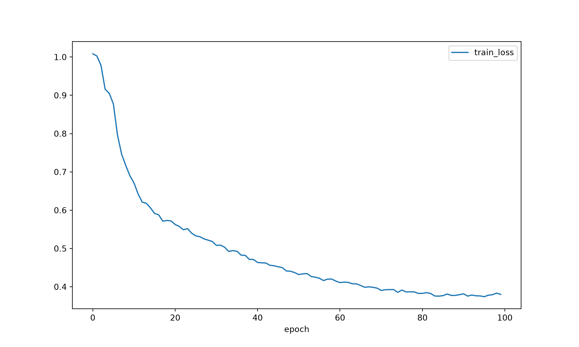
I next re-instantiate the FCMAE and load the saved parameters from the Lightning checkpoint. Since the model argument was excluded from the saved hyperparameters, it must be provided when the checkpoint is loaded.
litFCMAE = LitFCMAE.load_from_checkpoint("data/models/fcmaeVfill.ckpt",
                                         model=FCMAE(inChn=3), map_location="cpu")
27.4.4 Visualizing Reconstructions
Although the reconstruction loss is not the goal, visualizing the reconstructions is a useful check that pre-training is working. The function below masks an image, predicts the masked patches, and displays the original image, the masked input, and the reconstruction, in which the visible patches are copied from the input and the masked patches are predicted. If the normalized-pixel loss was used, the predicted patches are de-normalized using the mean and variance of the corresponding target patches so that they can be displayed on the same scale. The three LSPs are displayed as a false color composite. Expect the reconstructions to be blurry, especially after such a short pre-training process; they only need to capture the general structure of the masked regions.
def showReconstruction(model, img, bands=(0, 1, 2)):
    model.eval()
    with torch.no_grad():
        x = img.unsqueeze(0)
        _, pred, mask = model(x)
        p, C = model.p, model.inChn
        h, w = mask.shape[1:]
        if model.normPixLoss:
            target = patchify(x, p)
            pred = pred * (target.var(-1, keepdim=True) + 1e-6) ** 0.5 + target.mean(-1, keepdim=True)
        recon = unpatchify(pred, p, C, h, w)
        m = F.interpolate(mask.unsqueeze(1), scale_factor=p, mode="nearest")
        masked = x * (1 - m)
        combined = x * (1 - m) + recon * m

    def toRGB(t):
        a = t[0, list(bands)].permute(1, 2, 0).cpu().numpy()
        return np.clip((a - a.min()) / (a.max() - a.min() + 1e-6), 0, 1)

    fig, axs = plt.subplots(1, 3, figsize=(12, 4))
    for ax, t, title in zip(axs, [x, masked, combined], ["Original", "Masked", "Reconstruction"]):
        ax.imshow(toRGB(t)); ax.set_title(title); ax.axis("off")
plt.show()torch.manual_seed(42)
vizDS = UnlabeledChips(ssDF["chpPth"], augment=False)
showReconstruction(litFCMAE.model, vizDS[0])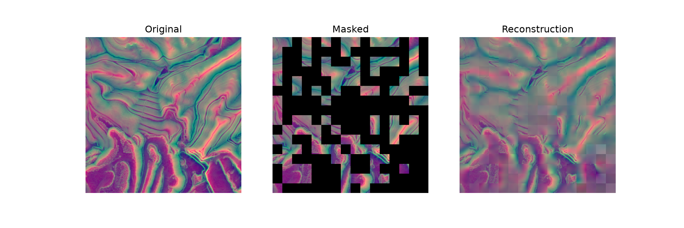
showReconstruction(litFCMAE.model, vizDS[1])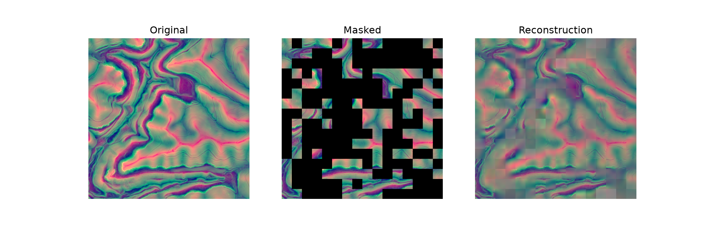
27.5 Using the Pre-Trained Encoder for Semantic Segmentation
In this section, I demonstrate how to build a UNet that uses the pre-trained encoder and how to set up the fine-tuning process, including setting different learning rates for each encoder stage and freezing and unfreezing the encoder. I do not train the segmentation model here. The training process is the same as the process demonstrated in Chapter 16 and Chapter 21, and the vfillDLMini chips and masks could be used to fine-tune the model to extract valley fill faces.
27.5.1 A UNet with the FCMAE Encoder
To use the pre-trained encoder for semantic segmentation, I define a UNet-like architecture that uses the ConvNeXt V2 encoder and a decoder similar to the one used in the ConvNeXt UNet from Chapter 24. The encoder provides feature maps at 1/4, 1/8, 1/16, and 1/32 of the input resolution. As with the ResNet and MobileNetV2 encoders in Chapter 17, the encoder does not provide features at the original resolution or at 1/2 resolution, since its stem reduces the spatial dimensions by a factor of 4. So, I add a small, randomly initialized convolutional stem that provides skip connections at full and half resolution. The decoder upsamples the features by a factor of 2 at each stage, concatenates the corresponding skip features, and applies a residual double convolution block with group normalization and GELU. The encoder is called without a mask, so it behaves as a standard ConvNeXt V2.
def gnGroups(nChn, groups=8):
    g = min(groups, nChn)
    while nChn % g:
        g -= 1
    return g

class ResDoubleConvGN(nn.Module):
    def __init__(self, inChn, outChn, groups=8):
        super().__init__()
        g = gnGroups(outChn, groups)
        self.f = nn.Sequential(
            nn.Conv2d(inChn, outChn, 3, padding=1, bias=False), nn.GroupNorm(g, outChn), nn.GELU(),
            nn.Conv2d(outChn, outChn, 3, padding=1, bias=False), nn.GroupNorm(g, outChn), nn.GELU())
        self.proj = nn.Sequential(nn.Conv2d(inChn, outChn, 1, bias=False), nn.GroupNorm(g, outChn))

    def forward(self, x):
        return self.f(x) + self.proj(x)

class UpBlock(nn.Module):
    def __init__(self, inChn, skipChn, outChn):
        super().__init__()
        self.conv = ResDoubleConvGN(inChn + skipChn, outChn)

    def forward(self, x, skip):
        x = F.interpolate(x, size=skip.shape[2:], mode="bilinear", align_corners=False)
        return self.conv(torch.cat([x, skip], dim=1))

class FCMAEUNet(nn.Module):
    def __init__(self, inChn=3, nCls=2, dims=(96, 192, 384, 768), depths=(2, 2, 6, 2),
                 decChn=(384, 192, 96, 64, 32), stemChn=(32, 64)):
        super().__init__()
        self.encoder = MaskedConvNeXtV2Encoder(inChn, dims, depths)
        self.stem1 = ResDoubleConvGN(inChn, stemChn[0])                                  # full resolution
        self.stem2 = nn.Sequential(nn.Conv2d(stemChn[0], stemChn[1], 3, stride=2, padding=1),
                                   ResDoubleConvGN(stemChn[1], stemChn[1]))               # 1/2 resolution
        skipChn = [dims[2], dims[1], dims[0], stemChn[1], stemChn[0]]
        inChns = [dims[3]] + list(decChn[:-1])
        self.ups = nn.ModuleList([UpBlock(i, s, o) for i, s, o in zip(inChns, skipChn, decChn)])
        self.head = nn.Conv2d(decChn[-1], nCls, kernel_size=1)

    def forward(self, x):
        s1 = self.stem1(x)
        s2 = self.stem2(s1)
        f4, f8, f16, f32 = self.encoder(x)
        y = f32
        for up, skip in zip(self.ups, [f16, f8, f4, s2, s1]):
            y = up(y, skip)
        return self.head(y)
Since the valley fill problem differentiates two classes (background and valley fill face), I set nCls to 2. Passing a random tensor with the shape of a vfillDLMini chip confirms that the model returns logits for each class at the original resolution.
segModel = FCMAEUNet(inChn=3, nCls=2)
print(segModel(torch.rand(1, 3, 512, 512)).shape)    # torch.Size([1, 2, 512, 512])
torch.Size([1, 2, 512, 512])27.5.2 Loading the Pre-Trained Parameters
Since the UNet’s encoder uses the same class as the FCMAE’s encoder, the saved parameters can be loaded directly into its encoder attribute. The stem, decoder, and head remain randomly initialized. The architecture settings (inChn, dims, and depths) must match those used for pre-training. The load_state_dict() method reports whether all of the keys matched. To confirm that the parameters were loaded, I compare one of the stem’s convolution weights to the corresponding weight in the FCMAE.
segModel = FCMAEUNet(inChn=3, nCls=2)
segModel.encoder.load_state_dict(torch.load("data/models/fcmaeVfillEncoder.pt",
                                            map_location="cpu"))
<All keys matched successfully>print(torch.equal(segModel.encoder.stem[0].weight, litFCMAE.model.encoder.stem[0].weight))True27.5.3 Freezing and Unfreezing the Encoder
As discussed in Chapter 13, the pre-trained parameters can be frozen so that they are not updated during training. A parameter is frozen by setting its requires_grad attribute to False, which stops PyTorch from calculating its gradient. Lightning’s BaseFinetuning class provides static methods for this purpose: freeze() freezes the parameters of one or more modules, and make_trainable() unfreezes them. These methods can be called outside of a training process. Below, I define a function to count the trainable parameters and then freeze and unfreeze the encoder.
def countTrainable(model):
    nTrain = sum(p.numel() for p in model.parameters() if p.requires_grad)
    nTotal = sum(p.numel() for p in model.parameters())
    print(f"Trainable parameters: {nTrain:,} of {nTotal:,}")

countTrainable(segModel)
Trainable parameters: 26,934,114 of 26,934,114BaseFinetuning.freeze(segModel.encoder)
countTrainable(segModel)Trainable parameters: 7,838,850 of 26,934,114BaseFinetuning.make_trainable(segModel.encoder)
countTrainable(segModel)Trainable parameters: 26,934,114 of 26,934,114Individual stages can also be frozen or unfrozen. To make this easier, the function below returns the modules associated with each encoder stage. I group the stem with the first stage and each downsampling layer with the stage that follows it. Below, I freeze the entire encoder and then unfreeze only the last stage, which is the stage that is generally unfrozen first.
def encoderStage(enc, i):
    return [enc.stem, enc.stages[0]] if i == 0 else [enc.downs[i - 1], enc.stages[i]]

BaseFinetuning.freeze(segModel.encoder)
BaseFinetuning.make_trainable(encoderStage(segModel.encoder, 3))
countTrainable(segModel)
Trainable parameters: 18,557,058 of 26,934,114BaseFinetuning.make_trainable(segModel.encoder)The freeze() method also places the frozen modules in evaluation mode so that the running means and variances of any batch normalization layers are not updated. Since the ConvNeXt V2 encoder uses layer normalization and GRN, which do not store running statistics, this is not a concern here.
27.5.4 Layer-Wise Learning Rates
As discussed in Chapter 13, a lower learning rate is generally used for the pre-trained encoder than for the randomly initialized components, and different learning rates are implemented using parameter groups. A common refinement for ConvNeXt and transformer encoders is layer-wise learning rate decay, in which each earlier stage of the encoder receives a smaller learning rate than the stage after it. The rationale is that the early stages learn generic features, such as edges and textures, that require little adjustment, while the later stages learn more task-specific features.
The function below builds the parameter groups. The four encoder stages receive learning rates that decrease by a factor of decay for each stage away from the decoder, while the stem, decoder, and head receive the full base learning rate. Only trainable parameters are included, so the function can also be used when some of the encoder stages are frozen. Each group is given a "name", which is used by Lightning’s LearningRateMonitor callback to label the logged learning rates.
def layerwiseParamGroups(model, baseLR=1e-3, decay=0.5):
    enc = model.encoder
    groups = []
    for i in range(4):
        params = [p for m in encoderStage(enc, i) for p in m.parameters() if p.requires_grad]
        if params:
            groups.append({"params": params, "lr": baseLR * decay ** (4 - i), "name": f"enc_stage{i+1}"})
    encIDs = {id(p) for p in enc.parameters()}
    groups.append({"params": [p for p in model.parameters() if id(p) not in encIDs and p.requires_grad],
                   "lr": baseLR, "name": "stem_decoder_head"})
    return groups
Printing the parameter groups of an AdamW optimizer confirms the learning rate assigned to each group and the number of parameters in each.
optimizer = torch.optim.AdamW(layerwiseParamGroups(segModel, baseLR=1e-3, decay=0.5), weight_decay=0.05)
for g in optimizer.param_groups:
    print(f'{g["name"]:<20} lr: {g["lr"]:.6f}  parameters: {sum(p.numel() for p in g["params"]):,}')
enc_stage1 lr: 0.000063 parameters: 164,832
enc_stage2 lr: 0.000125 parameters: 688,896
enc_stage3 lr: 0.000250 parameters: 7,523,328
enc_stage4 lr: 0.000500 parameters: 10,718,208
stem_decoder_head lr: 0.001000 parameters: 7,838,85027.5.5 Fine-Tuning with Lightning
The UNet can be fine-tuned using the LitSegmenter LightningModule from Chapter 16. To use layer-wise learning rates, I subclass it and override configure_optimizers() so that the optimizer is built from the parameter groups. A cosine schedule is applied to all of the groups, which maintains the ratios between their learning rates.
class LitFineTune(LitSegmenter):
    def __init__(self, model, nCls, criterion, lr=1e-3, decay=0.5):
        super().__init__(model, nCls, criterion, lr=lr)
        self.decay = decay

    def configure_optimizers(self):
        optimizer = torch.optim.AdamW(layerwiseParamGroups(self.model, self.lr, self.decay),
                                      weight_decay=0.05)
        scheduler = torch.optim.lr_scheduler.CosineAnnealingLR(optimizer, T_max=self.trainer.max_epochs)
        return {"optimizer": optimizer, "lr_scheduler": {"scheduler": scheduler, "interval": "epoch"}}
Freezing and unfreezing can be combined with layer-wise learning rates using gradual unfreezing and Lightning’s BaseFinetuning callback, as introduced in Chapter 13. In the callback below, the entire encoder is frozen before training begins, so only the randomly initialized stem, decoder, and head are updated. Starting at epoch startEpoch, one encoder stage is unfrozen every every epochs, beginning with the last stage. When a stage is unfrozen, its parameters are added to the optimizer as a new parameter group using unfreeze_and_add_param_group() with that stage’s layer-wise learning rate. Since layerwiseParamGroups() only includes trainable parameters, the frozen stages are not passed to the optimizer when training begins.
class GradualUnfreezeEncoder(BaseFinetuning):
    def __init__(self, baseLR=1e-3, decay=0.5, startEpoch=5, every=2):
        super().__init__()
        self.baseLR = baseLR
        self.decay = decay
        self.startEpoch = startEpoch
        self.every = every

    def freeze_before_training(self, pl_module):
        self.freeze(pl_module.model.encoder)

    def finetune_function(self, pl_module, current_epoch, optimizer):
        enc = pl_module.model.encoder
        for k, i in enumerate([3, 2, 1, 0]):                      # last stage first
            if current_epoch == self.startEpoch + k * self.every:
                self.unfreeze_and_add_param_group(encoderStage(enc, i), optimizer,
                                                  lr=self.baseLR * self.decay ** (4 - i))
Note that learning rate schedulers store the initial learning rate of each parameter group when they are created and do not adjust groups that are added later. So, when using gradual unfreezing, it is simplest to use a constant learning rate, as shown below, or to adjust the learning rates of the added groups manually.
class LitFineTuneUnfreeze(LitSegmenter):
    def __init__(self, model, nCls, criterion, lr=1e-3, decay=0.5):
        super().__init__(model, nCls, criterion, lr=lr)
        self.decay = decay

    def configure_optimizers(self):
        return torch.optim.AdamW(layerwiseParamGroups(self.model, self.lr, self.decay), weight_decay=0.05)
The code below shows how the fine-tuning process would be executed. Here, trainDL and valDL are DataLoaders that return the vfillDLMini chips and their masks, which could be built using the SegDataset class from Chapter 20. To use layer-wise learning rates without freezing, LitFineTune would be used and the GradualUnfreezeEncoder callback omitted.
from kornia import losses

segModel = FCMAEUNet(inChn=3, nCls=2)
segModel.encoder.load_state_dict(torch.load("data/models/fcmaeVfillEncoder.pt"))

litSeg = LitFineTuneUnfreeze(segModel, nCls=2, criterion=losses.DiceLoss(average="macro"),
                             lr=1e-3, decay=0.5)
trainer = L.Trainer(max_epochs=50, accelerator="gpu", devices=1, precision="bf16-mixed",
                    default_root_dir="data/output/",
                    callbacks=[GradualUnfreezeEncoder(baseLR=1e-3, decay=0.5, startEpoch=5, every=2),
                               ModelCheckpoint(monitor="val_f1", mode="max"),
                               LearningRateMonitor(logging_interval="epoch")])
trainer.fit(litSeg, train_dataloaders=trainDL, val_dataloaders=valDL)
27.6 Evaluating the Benefit of Pre-Training
Does self-supervised pre-training help? The answer depends on the amount of labeled data, the similarity between the pre-training and downstream data, and the amount of pre-training. The benefit is generally largest when labeled data are scarce. A useful experiment, sometimes called a label efficiency experiment, compares fine-tuned models initialized in different ways while varying the amount of labeled training data:
- Random initialization (training from scratch).
- FCMAE pre-training on your own unlabeled geospatial data.
- Other pre-trained weights, such as ImageNet ConvNeXt V2 weights (when the number of bands allows).
Each configuration is fine-tuned using, for example, 5%, 10%, 25%, and 100% of the labeled training chips, holding the validation and test data and all other settings constant, and the test-set metrics are compared. If pre-training is beneficial, the pre-trained models should outperform the randomly initialized model, especially with small training sets. Another common evaluation is linear probing, in which the encoder is frozen and only a simple head is trained, which directly measures the quality of the learned representations.
There are several reasons why domain-specific pre-training is attractive for geospatial data: it can use any number of input bands, such as multispectral bands or terrain variables, for which no ImageNet weights exist; it can use the spatial resolution and scale of the data to which the model will be applied; and it can exploit large unlabeled archives. Pre-training a model on a large and diverse geospatial dataset so that it can be fine-tuned for many downstream tasks is the idea behind the geospatial foundation models discussed in Chapter 28.
27.7 Concluding Remarks
In this chapter, we explored self-supervised pre-training using the fully convolutional masked autoencoder. We built a masked ConvNeXt V2 encoder and a lightweight decoder, pre-trained them to reconstruct masked patches of land surface parameter chips, and transferred the pre-trained encoder to a UNet-like architecture for semantic segmentation. We also demonstrated how to freeze and unfreeze the encoder and how to assign layer-wise learning rates to its stages for fine-tuning. In the next chapter, we explore foundation models, which apply this idea at a much larger scale, using the Segment Anything Model as an example.
27.8 Questions
- What is self-supervised learning? Explain the difference between a pretext task and a downstream task.
- Describe the masked autoencoder (MAE) pretext task. Why must a large proportion of the image be masked?
- Why is it more difficult to apply masked image modeling to CNNs than to transformers? How does the FCMAE address this problem?
- Explain the difference between sparse convolution and the dense masking approach used in this chapter. Do they produce the same outputs at the visible locations? Do they require the same amount of computation?
- Why is the FCMAE decoder intentionally lightweight? What is the purpose of the mask token?
- Why is the reconstruction loss calculated only for the masked patches? What is the purpose of normalizing the target pixels within each patch?
- Why is the reconstruction loss a poor indicator of the usefulness of the pre-trained encoder? How can the benefit of pre-training be evaluated?
- Explain layer-wise learning rate decay and gradual unfreezing. Why might they be beneficial when fine-tuning a pre-trained encoder?