import os
from functools import cache
from pathlib import Path

import numpy as np
import pandas as pd
import geopandas as gpd
from shapely.ops import unary_union
import rasterio as rio
from rasterio.mask import mask as rioMask
from rasterio.features import rasterize, geometry_mask
from rasterio.windows import Window
from rasterio.enums import Resampling
import matplotlib.pyplot as plt
from matplotlib.colors import ListedColormap, BoundaryNorm
from matplotlib.patches import Patch

import torch
from torch.utils.data import Dataset, DataLoader
import albumentations as A20 Creating Image Chips
20.1 Introduction
When applying deep learning to geospatial data, you will need to generate image chips and associated labels of a defined size to train the algorithm. In the case of semantic segmentation, each chip needs an associated pixel-level mask in which each class is assigned a unique numeric code. Multispectral imagery and other geospatial raster data commonly cover large spatial extents, so you will need to be able to “chip” these data into smaller, consistently sized subsets so that they can be used to train, validate, and assess deep learning models. As we saw in Chapter 19, the reverse process is used to make predictions over an entire extent: the data are broken into chips, each chip is predicted, and the predictions are reassembled into a single, continuous output.
There are two general approaches to generating chips:
- Static chips are generated once, before training, and saved to disk. The DataSet reads the saved chips. This is the approach we have used throughout this text.
- Dynamic chips are generated during training. A table stores the locations at which chips should be extracted, and each chip and its mask are generated from the original raster and vector data when the chip is requested by the DataLoader.
In this chapter, I demonstrate both approaches. Instead of relying on a package, I define all of the chip generation functions in the chapter using Rasterio, GeoPandas, and NumPy so that you can see how each step works and modify the functions for your own data. The workflow mirrors the one implemented by our geodl R package, which is discussed in our Geospatial Supervised Learning using R text, and by the terrainseg Python package, which my lab group developed for terrain data. The functions defined here work with multiband data and add a few conveniences, such as a single function for binary and multiclass chips, flagging unlabeled areas as NoData in the masks, and random jitter for dynamic chips. Other options for generating chips include TorchGeo, which provides geospatial DataSets and samplers for PyTorch; the Export Training Data for Deep Learning tool in ArcGIS Pro; and the Produce Training Data for Deep Learning plugin for QGIS.
I begin by importing the required libraries.
I define the folder that contains the input data, which are provided in the data/files/chipGen folder, and the folder to which output will be written.
fldPth = "data/files/chipGen/"
outPth = "data/output/"
20.2 Static Chips
20.2.1 Input Data
For this demonstration, I use a subset of an image from the Landcover.ai dataset, which was used in Chapter 16, along with three vector datasets: the extent of the labeled area, building footprints, and a wall-to-wall land cover classification. For the land cover data, every area within the extent is labeled to one of five classes: background, building, woodland, water, or road. These classes are coded 0 through 4 in the “gridcode” attribute. For the building footprints, the “gridcode” attribute is 1 for all features.
The image extent is irregularly shaped. Areas outside of the labeled extent are stored as NoData. The extent is important because areas outside of it cannot be assumed to be background: they simply have not been interpreted.
ext = gpd.read_file(fldPth + "extent.shp")
buildings = gpd.read_file(fldPth + "buildingsPolys.shp")
lc = gpd.read_file(fldPth + "mskPoly.shp")

cNamesLC = ["Background", "Building", "Woodland", "Water", "Road"]
cColorsLC = ["gray", "red", "green", "blue", "black"]

fig, axs = plt.subplots(1, 3, figsize=(12, 6))
with rio.open(fldPth + "img.tif") as src:
    img = src.read(masked=True)
axs[0].imshow(np.transpose(img, (1, 2, 0)).filled(255).astype("uint8"))
axs[0].set_title("Image")
ext.boundary.plot(ax=axs[1], color="red", linewidth=2)
buildings.plot(ax=axs[1], color="gray")
axs[1].set_title("Buildings")
ext.boundary.plot(ax=axs[2], color="red", linewidth=2)
lc.plot(ax=axs[2], column="gridcode", cmap=ListedColormap(cColorsLC), categorical=True)
axs[2].set_title("Land Cover")
for ax in axs:
    ax.set_axis_off()
plt.show()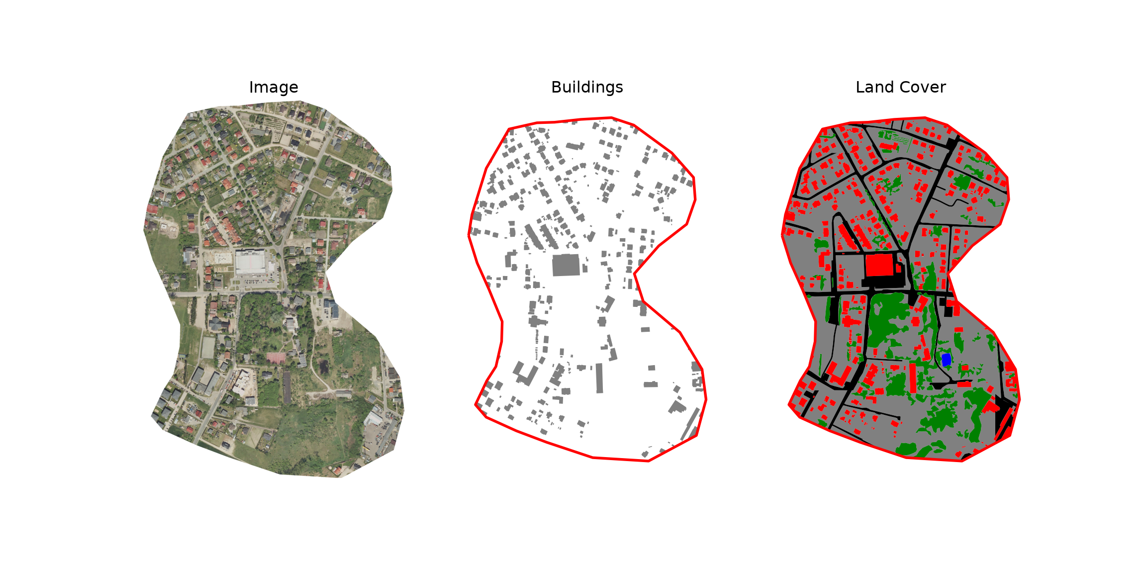
20.2.2 Create Masks
The first step is to convert the vector features into a raster mask that is aligned with the raster grid. The makeMask() function defined below rasterizes the vector features to a categorical raster that has the same cell size, coordinate reference system, and extent as the reference raster. Its arguments are:
-
image: path to the reference raster, which defines the grid of the output mask. -
features: path to the vector features to rasterize. -
outMask: output file path for the mask. -
field: the attribute column that stores the numeric class code to burn into the mask. IfNone, all features are coded to 1. -
background: the code assigned to cells not covered by any feature (0 by default). -
extent: optional path to a polygon file defining the labeled extent. If provided, the image and mask are cropped to the extent, and mask cells outside of the extent are assigned themaskNoDatavalue (255 by default) so that unlabeled areas are not mistaken for background. -
outImage: optional output file path for the cropped image. If an extent is used, the cropped image should be written at least once so that the image and mask have the same extent and number of rows and columns. -
allTouched: ifFalse, only cells whose centers fall within a feature are burned. IfTrue, all cells touched by a feature are burned, which can be useful for small or thin features.
The function works as follows. The features, and extent if provided, are read and projected to the coordinate reference system of the raster if necessary. If an extent is provided, the raster is cropped to it using rasterio.mask.mask(), which also sets cells outside of the extent polygon(s) to NoData. The features are then rasterized to the (possibly cropped) grid using rasterize(), and geometry_mask() is used to flag cells outside of the extent. Lastly, the image and mask are written to GeoTIFF files using the profile of the source raster, updated to reflect the cropped dimensions and transform.
def makeMask(image, features, outMask, field=None, background=0, extent=None,
             outImage=None, maskNoData=255, allTouched=False):
    with rio.open(image) as src:
        feats = gpd.read_file(features).to_crs(src.crs)
        profile = src.profile.copy()
        if extent is not None:
            extGeoms = list(gpd.read_file(extent).to_crs(src.crs).geometry)
            imgNoData = src.nodata if src.nodata is not None else 0
            img, transform = rioMask(src, extGeoms, crop=True, nodata=imgNoData)
            profile.update(nodata=imgNoData)
        else:
            img, transform = src.read(), src.transform
    shape = img.shape[1:]
    profile.update(height=shape[0], width=shape[1], transform=transform)

    values = feats[field] if field is not None else [1] * len(feats)
    msk = rasterize(zip(feats.geometry, values), out_shape=shape, transform=transform,
                    fill=background, all_touched=allTouched, dtype="uint8")
    if extent is not None:
        outside = geometry_mask(extGeoms, out_shape=shape, transform=transform)
        msk[outside] = maskNoData

    if outImage is not None:
        with rio.open(outImage, "w", **profile) as dst:
            dst.write(img)
    mskProfile = profile.copy()
    mskProfile.update(count=1, dtype="uint8",
                      nodata=maskNoData if extent is not None else None)
    with rio.open(outMask, "w", **mskProfile) as dst:
        dst.write(msk, 1)
Codes should be assigned from 0 to the number of classes minus 1 without skipping values. For a binary classification, the background should be coded to 0 and the positive class to 1. Since the mask is stored as an unsigned 8-bit integer, up to 255 classes can be differentiated, with the value 255 reserved for NoData.
For the binary building problem, I crop to the extent and write both a copy of the image and the mask. Since all building features have a “gridcode” of 1 and the background is assigned 0, the resulting mask contains values of 0 and 1 within the extent and 255 outside of it.
makeMask(image=fldPth + "img.tif",
         features=fldPth + "buildingsPolys.shp",
         outMask=outPth + "buildingMskOut.tif",
         field="gridcode",
         background=0,
         extent=fldPth + "extent.shp",
         outImage=outPth + "imgOut.tif")
For the multiclass land cover problem, the setup is the same except that I only write the mask since the cropped image was already created above. The background value of 0 is not used in this case since the polygons completely fill the labeled extent.
makeMask(image=fldPth + "img.tif",
         features=fldPth + "mskPoly.shp",
         outMask=outPth + "lcMskOut.tif",
         field="gridcode",
         background=0,
         extent=fldPth + "extent.shp")
I next read the two masks back in and display them. Since they are categorical data, I use a BoundaryNorm so that each class code is mapped to a single color. Reading the masks with masked=True returns a masked array in which the NoData cells outside of the extent are masked, so they are displayed as transparent.
def plotMask(ax, msk, cColors, title):
    nCls = len(cColors)
    norm = BoundaryNorm(np.arange(-0.5, nCls), nCls)
    ax.imshow(msk, cmap=ListedColormap(cColors), norm=norm, interpolation="nearest")
    ax.set_title(title)
    ax.set_axis_off()

with rio.open(outPth + "buildingMskOut.tif") as src:
    mskB = src.read(1, masked=True)
with rio.open(outPth + "lcMskOut.tif") as src:
    mskLC = src.read(1, masked=True)

fig, axs = plt.subplots(1, 2, figsize=(10, 7))
plotMask(axs[0], mskB, ["gray", "red"], "Buildings")
plotMask(axs[1], mskLC, cColorsLC, "Land Cover")
fig.legend(handles=[Patch(facecolor=c, label=n) for c, n in zip(cColorsLC, cNamesLC)],
           loc="lower center", ncol=5, frameon=False)
plt.show()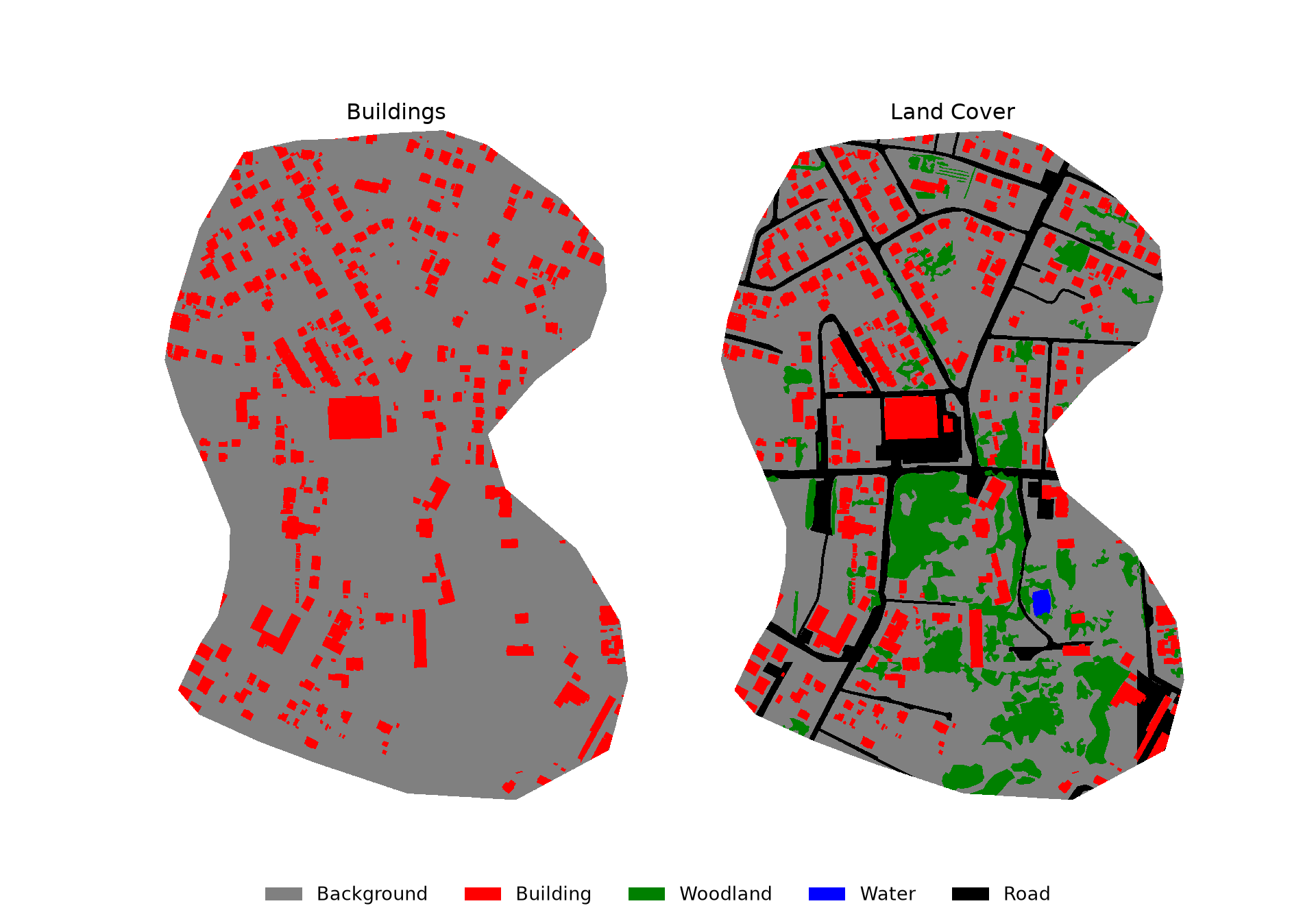
20.2.3 Make Chips
Once raster masks have been generated that align with the predictor variables, they can be broken into chips of a defined size using the makeChips() function defined below. Its arguments are:
-
imageandmask: paths to the image and mask, which must have the same extent, cell size, number of rows and columns, and coordinate reference system. -
outDir: the output directory. “images” and “masks” subfolders are created within this directory. -
size: the height and width of the chips in pixels (e.g., 128, 256, or 512). -
strideXandstrideY: the distance, in pixels, that the moving window moves in the x and y directions as the chips are generated. If the strides equal the chip size, the chips do not overlap. Smaller strides produce overlapping chips, which increases the number of chips, but overlapping chips are highly correlated. Larger strides leave gaps between chips. If not specified, the strides are set equal tosize. -
bands: the bands to include in the chips, numbered from 1. IfNone, all bands are included. -
mode: which chips to write."All"writes all chips, including those that contain no cells mapped to a positive class."Positive"writes only chips that contain at least one cell that is not coded as background."Divided"writes all chips but saves background-only chips to “background” subfolders and chips that contain at least one positive cell to “positive” subfolders. -
background: the code used for the background class, which is used by the"Positive"and"Divided"modes.
The "Divided" mode is especially useful for binary problems with class imbalance, since it makes it easy to use only a subset of the background-only chips during training, as we will do in Chapter 21. The same function is used for binary and multiclass problems. For multiclass problems, "All" is generally used, since every class code other than the background is treated as a “positive” class by the other modes.
The function first checks that the image and mask grids align. It then calculates the row and column offsets of the upper-left corner of each chip. If the chips do not evenly divide the raster, a final row and column of chips is added that is aligned with the bottom and right edges of the raster so that the entire grid is covered. Each chip and mask are read using a Rasterio Window. Only complete chips are written: read_masks() and dataset_mask() return arrays in which NoData cells are coded to 0, and any chip that contains a NoData cell in the image or mask is skipped, which is important here since the image is irregularly shaped. Each chip is written with its own transform, calculated using window_transform(), so that the chips retain their spatial reference information and can be viewed in a GIS. The chips are named using the name of the source image and the row and column offsets of the chip, so chips generated from multiple images can be written to the same folder. Since existing chips are not deleted, you should write to an empty folder or delete the old chips if you regenerate them with different settings. The function returns the number of chips written.
def chipOffsets(length, size, stride):
    offsets = list(range(0, length - size + 1, stride))
    if offsets[-1] != length - size:
        offsets.append(length - size)
    return offsets

def makeChips(image, mask, outDir, size=256, strideX=None, strideY=None, bands=None,
              mode="All", background=0):
    if mode not in ("All", "Positive", "Divided"):
        raise ValueError("mode must be 'All', 'Positive', or 'Divided'.")
    strideX = strideX or size
    strideY = strideY or size
    subDirs = ["positive", "background"] if mode == "Divided" else [""]
    for d in ("images", "masks"):
        for s in subDirs:
            os.makedirs(os.path.join(outDir, d, s), exist_ok=True)
    base = os.path.splitext(os.path.basename(image))[0]
    cnt = 0
    with rio.open(image) as srcImg, rio.open(mask) as srcMsk:
        if (srcImg.shape != srcMsk.shape or srcImg.transform != srcMsk.transform
                or srcImg.crs != srcMsk.crs):
            raise ValueError("The image and mask grids do not align.")
        bands = bands or list(range(1, srcImg.count + 1))
        imgProfile = srcImg.profile.copy()
        imgProfile.update(width=size, height=size, count=len(bands))
        mskProfile = srcMsk.profile.copy()
        mskProfile.update(width=size, height=size, count=1)
        for r in chipOffsets(srcImg.height, size, strideY):
            for c in chipOffsets(srcImg.width, size, strideX):
                window = Window(c, r, size, size)
                imgValid = srcImg.read_masks(bands, window=window)
                mskValid = srcMsk.dataset_mask(window=window)
                if (imgValid == 0).any() or (mskValid == 0).any():
                    continue
                msk = srcMsk.read(1, window=window)
                isPositive = bool((msk != background).any())
                if mode == "Positive" and not isPositive:
                    continue
                sub = ("positive" if isPositive else "background") if mode == "Divided" else ""
                name = f"{base}_{r}_{c}.tif"
                transform = srcImg.window_transform(window)
                with rio.open(os.path.join(outDir, "images", sub, name), "w",
                              **{**imgProfile, "transform": transform}) as dst:
                    dst.write(srcImg.read(bands, window=window))
                with rio.open(os.path.join(outDir, "masks", sub, name), "w",
                              **{**mskProfile, "transform": transform}) as dst:
                    dst.write(msk, 1)
                cnt += 1
    return cnt
For the building example, I generate 512x512 pixel chips with no overlap and only write chips that contain building pixels.
makeChips(image=outPth + "imgOut.tif",
          mask=outPth + "buildingMskOut.tif",
          outDir=outPth + "bChips/",
          size=512,
          strideX=512,
          strideY=512,
mode="Positive")12For the multiclass problem, I use the "All" mode, so all complete chips are written.
makeChips(image=outPth + "imgOut.tif",
          mask=outPth + "lcMskOut.tif",
          outDir=outPth + "lcChips/",
          size=512,
          strideX=512,
          strideY=512,
mode="All")1220.2.4 Make Chips DataFrame
Once chips have been created, they can be listed in a DataFrame using the makeChipsDF() function defined below. The mode argument must match the mode used to generate the chips. The “chpN” column provides the name of each chip while the “chpPth” and “mskPth” columns provide the paths to the image chip and mask, respectively. If the "Divided" mode was used, a “division” column indicates whether each chip is a background-only or positive case-containing sample. The paths are built from the folder path provided using pathlib, with forward slashes as separators on all operating systems, so if a relative path is used, as is the case here, the table can still be used if the project folder is moved to a new location or computer. The table can optionally be shuffled using the shuffle and seed arguments and saved to a CSV file by providing a path to the outCSV argument.
def makeChipsDF(folder, mode="All", extension=".tif", shuffle=False, seed=None, outCSV=None):
    if mode not in ("All", "Positive", "Divided"):
        raise ValueError("mode must be 'All', 'Positive', or 'Divided'.")
    subDirs = {"Positive": "positive", "Background": "background"} if mode == "Divided" else {None: ""}
    dfs = []
    for division, sub in subDirs.items():
        imgDir, mskDir = Path(folder, "images", sub), Path(folder, "masks", sub)
        chips = sorted(f.name for f in imgDir.iterdir() if f.suffix.lower() == extension.lower())
        df = pd.DataFrame({"chpN": chips,
                           "chpPth": [(imgDir / f).as_posix() for f in chips],
                           "mskPth": [(mskDir / f).as_posix() for f in chips]})
        if division is not None:
            df["division"] = division
        dfs.append(df)
    df = pd.concat(dfs, ignore_index=True)
    if shuffle:
        df = df.sample(frac=1, random_state=seed).reset_index(drop=True)
    if outCSV is not None:
        df.to_csv(outCSV, index=False)
    return df
Each table contains 12 chips. Note that, although the input image is much larger, many potential chips were not written because they include areas outside of the labeled extent, and, for the building chips, because they do not contain any building pixels.
bChipsDF = makeChipsDF(outPth + "bChips/", mode="Positive")
lcChipsDF = makeChipsDF(outPth + "lcChips/", mode="All")

print(len(bChipsDF), len(lcChipsDF))
12 12bChipsDF.head() chpN ... mskPth
0 imgOut_1024_1024.tif ... data/output/bChips/masks/imgOut_1024_1024.tif
1 imgOut_1024_512.tif ... data/output/bChips/masks/imgOut_1024_512.tif
2 imgOut_1536_1024.tif ... data/output/bChips/masks/imgOut_1536_1024.tif
3 imgOut_1536_512.tif ... data/output/bChips/masks/imgOut_1536_512.tif
4 imgOut_2048_1024.tif ... data/output/bChips/masks/imgOut_2048_1024.tif
[5 rows x 3 columns]20.2.5 View Chips
It is always a good idea to visualize a random subset of the chips to make sure that they were generated as expected and that the masks align with the images. The function below plots a random sample of chips from a chips DataFrame, with each image displayed above its mask. The user specifies the code (cCodes), name (cNames), and color (cColors) of each class. The prepDisplay() helper function applies a 2% to 98% percentile stretch to each chip so that it can be displayed by matplotlib. The first three bands are displayed as an RGB composite, and single-band data, such as DTMs, are displayed in grayscale.
def prepDisplay(img):
    img = img[:3] if img.shape[0] >= 3 else np.repeat(img[:1], 3, axis=0)
    lo, hi = np.percentile(img, [2, 98])
    return np.clip((img - lo) / (hi - lo + 1e-8), 0, 1).transpose(1, 2, 0)

def plotChipGrid(images, masks, cCodes, cNames, cColors, nCols=5):
    n = len(images)
    nCols = min(nCols, n)
    nRows = int(np.ceil(n / nCols))
    cmap = ListedColormap(cColors)
    norm = BoundaryNorm(np.append(np.array(cCodes) - 0.5, cCodes[-1] + 0.5), len(cCodes))
    fig, axs = plt.subplots(nRows * 2, nCols, figsize=(nCols * 2.5, nRows * 5), squeeze=False)
    for i in range(n):
        r, c = (i // nCols) * 2, i % nCols
        axs[r, c].imshow(prepDisplay(images[i]))
        axs[r + 1, c].imshow(masks[i], cmap=cmap, norm=norm, interpolation="nearest")
    for ax in axs.flatten():
        ax.set_axis_off()
    fig.legend(handles=[Patch(facecolor=cl, label=nm) for cl, nm in zip(cColors, cNames)],
               loc="lower center", ncol=len(cNames), frameon=False)
    plt.show()

def viewChips(chpDF, nSamps, cCodes, cNames, cColors, nCols=5, seed=42):
    samp = chpDF.sample(n=min(nSamps, len(chpDF)), random_state=seed)
    images, masks = [], []
    for _, row in samp.iterrows():
        with rio.open(row["chpPth"]) as src:
            images.append(src.read().astype("float32"))
        with rio.open(row["mskPth"]) as src:
            masks.append(src.read(1))
    plotChipGrid(images, masks, cCodes, cNames, cColors, nCols)
viewChips(bChipsDF, nSamps=10, cCodes=[0, 1], cNames=["Background", "Building"],
cColors=["gray", "red"])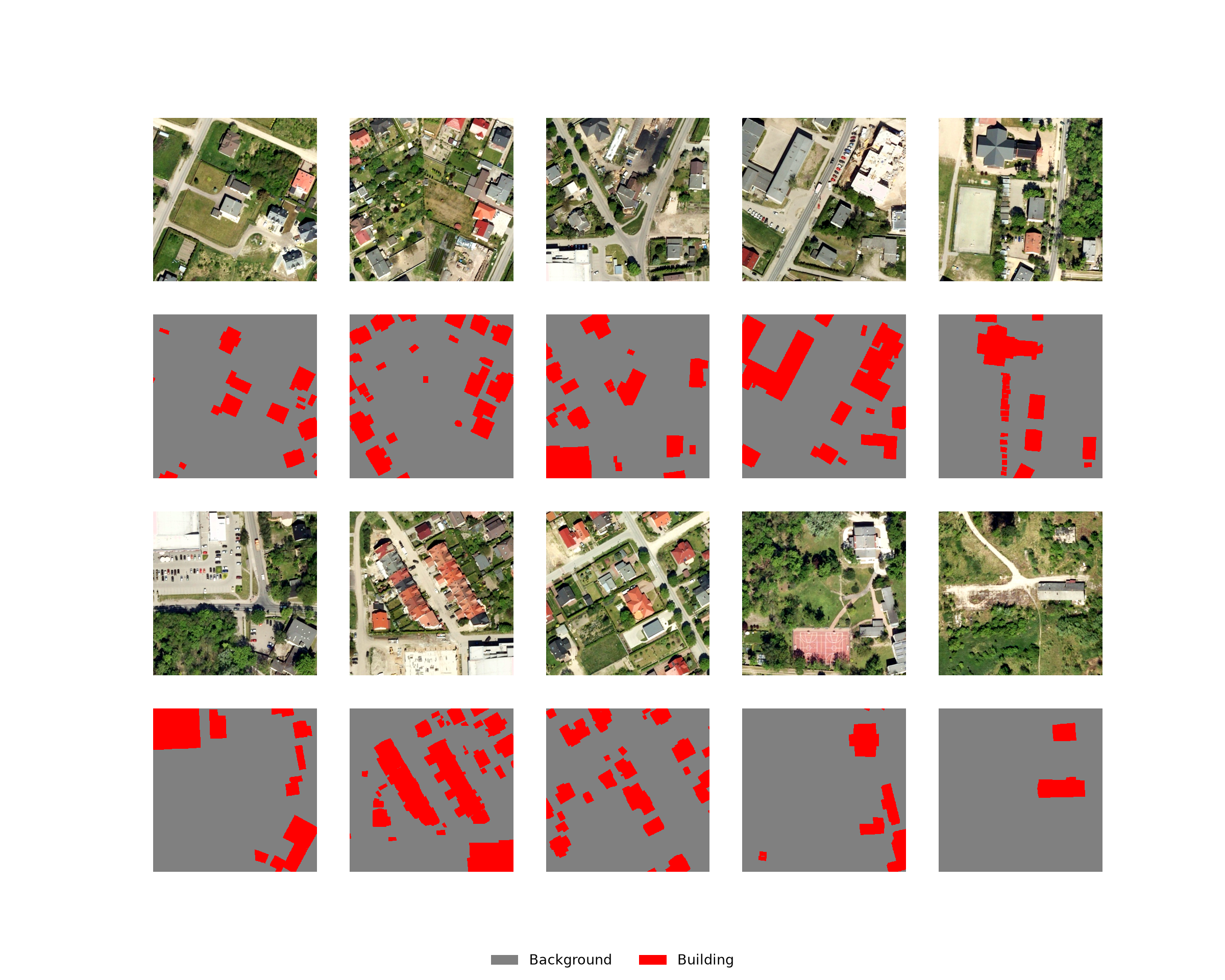
viewChips(lcChipsDF, nSamps=10, cCodes=[0, 1, 2, 3, 4], cNames=cNamesLC, cColors=cColorsLC)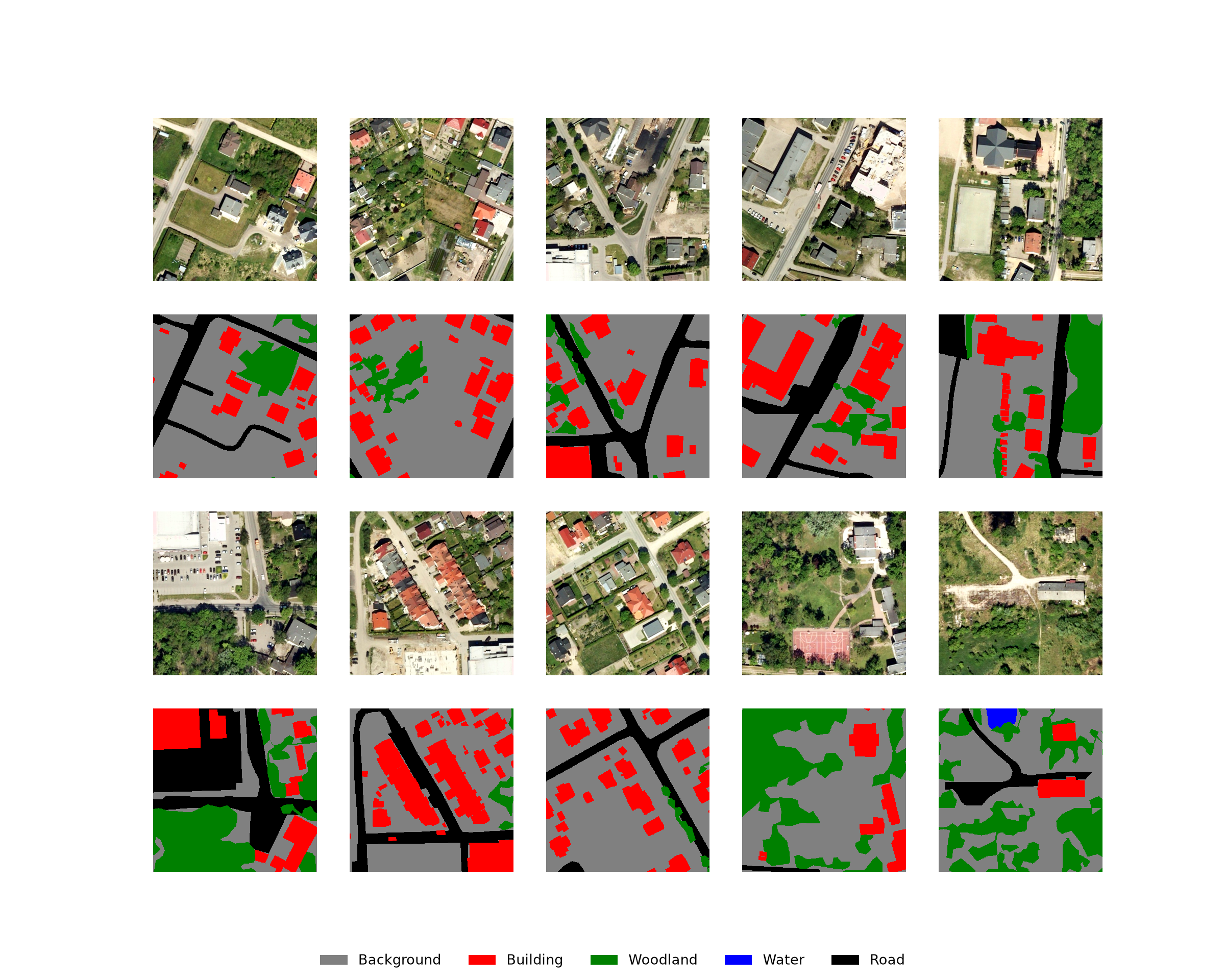
20.2.6 DataSets and DataLoaders
To use the chips to train a model, a DataSet subclass is needed that reads a chip and its mask, applies optional data augmentations, and returns tensors. The class below reads the requested bands of each chip using Rasterio and rescales them to a 0 to 1 scale by dividing by rescaleFactor, which is 255 here since the data are 8-bit. Albumentations transforms are applied to the image and mask together so that geometric augmentations, such as flips and rotations, do not break their alignment. Changes in brightness, contrast, and saturation are only applied to the image. The image is returned as a 32-bit float tensor with a shape of (C, H, W), and the mask is returned as a long integer tensor with a shape of (H, W). This is the same pattern discussed in Chapter 5.
class SegDataset(Dataset):
    def __init__(self, chpDF, bands=(1, 2, 3), rescaleFactor=255.0, transform=None):
        self.chpDF = chpDF.reset_index(drop=True)
        self.bands = list(bands)
        self.rescaleFactor = rescaleFactor
        self.transform = transform

    def __getitem__(self, idx):
        row = self.chpDF.iloc[idx]
        with rio.open(row["chpPth"]) as src:
            image = src.read(self.bands).astype("float32") / self.rescaleFactor
        with rio.open(row["mskPth"]) as src:
            mask = src.read(1).astype("int64")
        return toTensors(image, mask, self.transform)

    def __len__(self):
        return len(self.chpDF)

def toTensors(image, mask, transform=None):
    image = np.transpose(image, (1, 2, 0))
    if transform is not None:
        out = transform(image=image, mask=mask)
        image, mask = out["image"], out["mask"]
    image = torch.from_numpy(np.ascontiguousarray(np.transpose(image, (2, 0, 1))))
    mask = torch.from_numpy(np.ascontiguousarray(mask)).long()
    return image, mask
The toTensors() helper function applies the augmentations and converts the arrays to tensors. It is defined separately so that it can be reused by the dynamic chip DataSet defined later in the chapter.
The flips and rotations are applied with a 30% probability, brightness and contrast changes with a 10% probability, and saturation changes with a 20% probability. Not all augmentations are appropriate for all data types. For example, hue and saturation adjustments are only applicable to RGB data.
I use a mini-batch size of 5, shuffle the chips, and drop the last mini-batch since it may be incomplete if the number of chips is not divisible by the mini-batch size.
trainTransform = A.Compose([
    A.VerticalFlip(p=0.3),
    A.HorizontalFlip(p=0.3),
    A.RandomRotate90(p=0.3),
    A.RandomBrightnessContrast(brightness_limit=0.2, contrast_limit=0.2, p=0.1),
    A.HueSaturationValue(hue_shift_limit=0, sat_shift_limit=20, val_shift_limit=0, p=0.2),
])

bDS = SegDataset(bChipsDF, transform=trainTransform)
lcDS = SegDataset(lcChipsDF, transform=trainTransform)

bDL = DataLoader(bDS, batch_size=5, shuffle=True, drop_last=True)
lcDL = DataLoader(lcDS, batch_size=5, shuffle=True, drop_last=True)

print(len(bDL), len(lcDL))
2 220.2.7 Check Mini-Batches
Before training, it is also good practice to check the mini-batches generated by the DataLoader. The viewBatch() function below plots a mini-batch of images and masks using the same plotting function as viewChips(), and the describeBatch() function returns summary information: the number of samples, the data types and shapes of the image and mask tensors, the band means and standard deviations, the number of cells mapped to each class, and the minimum and maximum class codes. Catching problems at this stage, such as incorrect data types, unexpected class codes, or misaligned masks, is much better than discovering them after a long training process.
def viewBatch(dataLoader, cCodes, cNames, cColors, nCols=5):
    images, masks = next(iter(dataLoader))
    plotChipGrid(images.numpy(), masks.numpy(), cCodes, cNames, cColors, nCols)

def describeBatch(dataLoader, nCls):
    images, masks = next(iter(dataLoader))
    return {"batchSize": images.shape[0],
            "imageDataType": images.dtype,
            "maskDataType": masks.dtype,
            "imageShape": tuple(images.shape),
            "maskShape": tuple(masks.shape),
            "bndMns": images.mean(dim=(0, 2, 3)).numpy().round(4),
            "bndSDs": images.std(dim=(0, 2, 3)).numpy().round(4),
            "maskCount": torch.bincount(masks.flatten(), minlength=nCls).numpy(),
            "minIndex": masks.min().item(),
            "maxIndex": masks.max().item()}
viewBatch(bDL, cCodes=[0, 1], cNames=["Background", "Building"], cColors=["gray", "red"])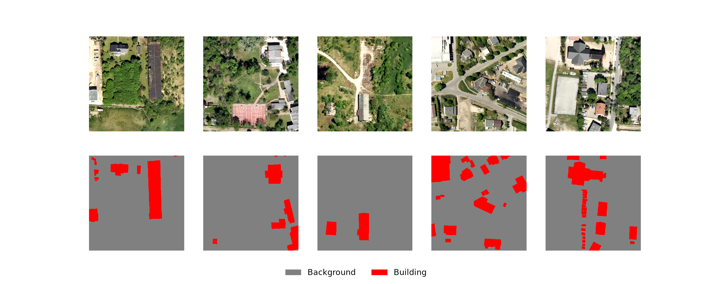
describeBatch(bDL, nCls=2){'batchSize': 5, 'imageDataType': torch.float32, 'maskDataType': torch.int64, 'imageShape': (5, 3, 512, 512), 'maskShape': (5, 512, 512), 'bndMns': array([0.5203, 0.521 , 0.4321], dtype=float32), 'bndSDs': array([0.1654, 0.1433, 0.1498], dtype=float32), 'maskCount': array([1165120, 145600]), 'minIndex': 0, 'maxIndex': 1}viewBatch(lcDL, cCodes=[0, 1, 2, 3, 4], cNames=cNamesLC, cColors=cColorsLC)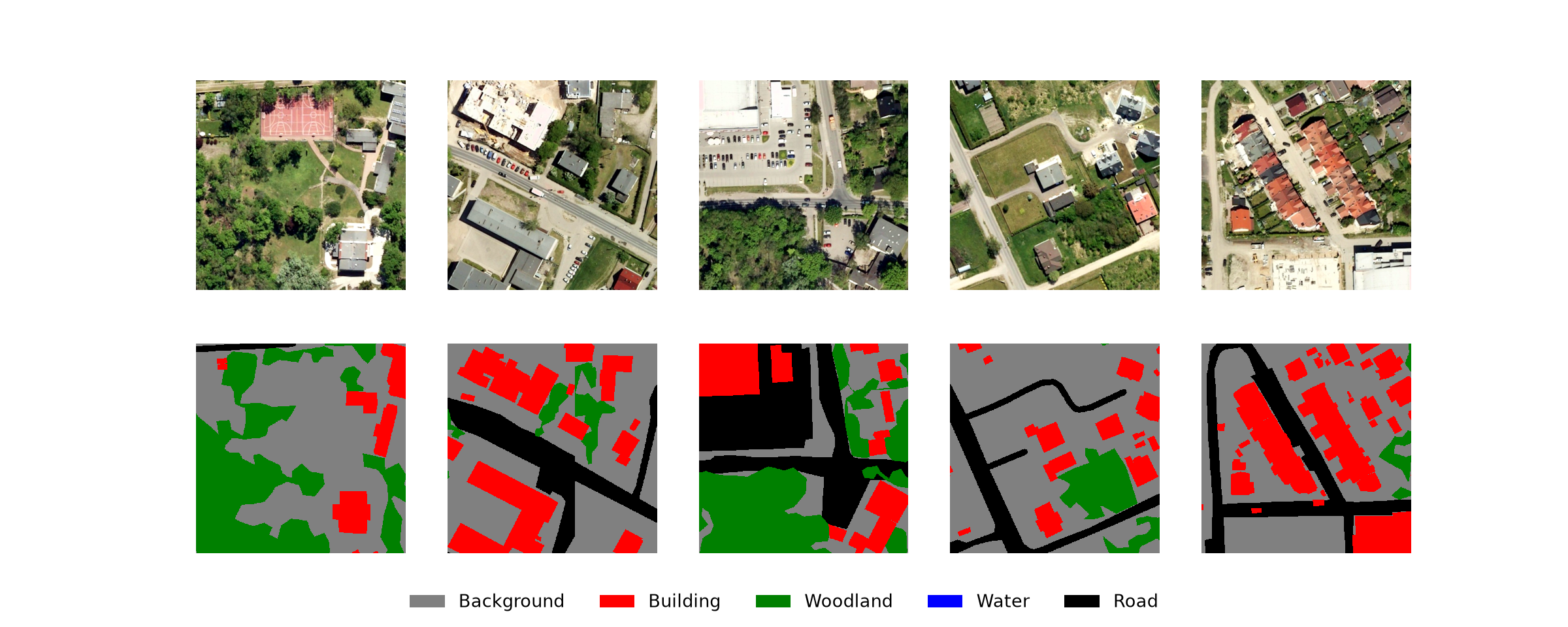
describeBatch(lcDL, nCls=5){'batchSize': 5, 'imageDataType': torch.float32, 'maskDataType': torch.int64, 'imageShape': (5, 3, 512, 512), 'maskShape': (5, 512, 512), 'bndMns': array([0.516, 0.521, 0.437], dtype=float32), 'bndSDs': array([0.1712, 0.1513, 0.1612], dtype=float32), 'maskCount': array([657674, 189008, 292105, 0, 171933]), 'minIndex': 0, 'maxIndex': 4}20.3 Dynamic Chips
Static chips have several disadvantages. They require disk space and time to generate, and they lock in a single chip size, cell size, and set of chip locations. If you want to experiment with a different chip size or with different input variables, the chips must be regenerated. Dynamic chips avoid these issues. Instead of saving chips to disk, you define a table of chip center locations, and the DataSet extracts each chip from the original raster and rasterizes its mask from the original vector data when the chip is requested. This allows:
- Changing the chip size or cell size without regenerating data.
- Sampling chips centered on the features of interest, which ensures that features are not split across chip edges and gives more control over class balance.
- Adding background chips by sampling random locations within the labeled extent.
- Swapping the predictor raster grid, for example, to experiment with different input variables, using the same chip locations and labels.
- Randomly shifting, or jittering, the chip centers during training, so that each feature appears at a slightly different position each time it is sampled.
The disadvantage is that generating chips from the original data during training is slower than reading small, pre-generated chips, especially for very large raster grids or vector datasets. Storing the data on a solid-state drive and using multiple DataLoader workers can help.
20.3.1 Input Data
The problem explored in this section is extracting valley fill faces resulting from surface coal mining reclamation from digital terrain models (DTMs). All valley fill faces within three study areas, two in eastern Kentucky and one in southwestern Virginia, USA, have been mapped. For each study area, there is a DTM with a 2 m cell size, a polygon file of the mapped valley fill faces, and a polygon file of the extent. The valley fill polygons contain a “code” attribute that stores a value of 1 for all features since there is only one class being differentiated.
These data are large and are not provided with the book download. They are part of the vfillDL dataset, which can be downloaded from figshare. I store the information for each study area in a DataFrame.
ImportantData Location
This section uses the vfillDL dataset, which is too large to include in the book download and must be downloaded from the source listed in Table 2. By default, the code expects the uncompressed vfillDL folder, which contains the dems, extents, and vectors folders, to be saved in the data/files folder (data/files/vfillDL). If you saved the data elsewhere, set vfPth below to the folder’s location on your machine.
# Set this to the location of the uncompressed vfillDL folder on your machine.
vfPth = "data/files/vfillDL/"

areas = pd.DataFrame({"name": ["KY1", "KY2", "VA1"],
                      "dem": ["ky1_dem.tif", "ky_2_dem.tif", "va1_dem.tif"]})
Below, I plot the three extents and the centroids of the valley fill faces.
allExtents = pd.concat([gpd.read_file(f"{vfPth}extents/testing{n}.shp") for n in areas["name"]])
allFeatures = pd.concat([gpd.read_file(f"{vfPth}vectors/testing{n}.shp") for n in areas["name"]])

fig, ax = plt.subplots(figsize=(8, 6))
allExtents.boundary.plot(ax=ax, color="black", linewidth=2)
allFeatures.centroid.plot(ax=ax, color="red", markersize=4)
ax.set_title("Study Areas and Valley Fill Faces")
plt.show()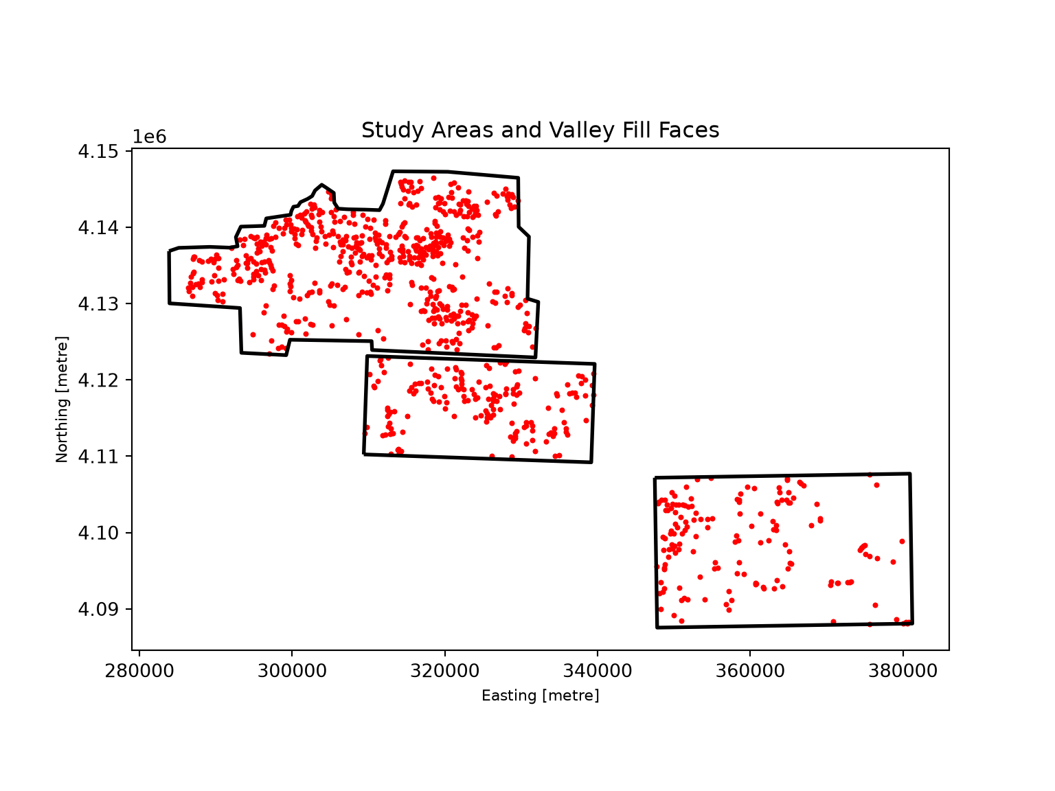
20.3.2 Define Chip Centers
The chips will be centered on the valley fill faces, so I first convert the polygons to points at their centroids. If chips are always centered exactly on a feature, the model will always see the features at the center of the chips, which is not the case when making predictions over an entire extent. So, I add random Gaussian noise, with a standard deviation of 20 m, to the coordinates of each point using the addCoordNoise() function defined below. The points for each study area are then saved to disk.
def addCoordNoise(gdf, amount, seed=None):
    rng = np.random.default_rng(seed)
    out = gdf.copy()
    out["geometry"] = gpd.points_from_xy(out.geometry.x + rng.normal(0, amount, len(out)),
                                         out.geometry.y + rng.normal(0, amount, len(out)),
                                         crs=out.crs)
    return out

for n in areas["name"]:
    vf = gpd.read_file(f"{vfPth}vectors/testing{n}.shp")
    vfP = vf[["code", "geometry"]].copy()
    vfP["geometry"] = vfP.centroid
    addCoordNoise(vfP, amount=20, seed=42).to_file(f"{outPth}{n.lower()}P.shp")
The makeDynamicChipsGDF() function defined below builds a GeoDataFrame of chip center locations. The centers can be provided as points or polygons; if polygons are provided, their centroids are used. The centers and masks are defined by separate datasets: here, the chips are centered on the noisy centroids, while the masks are generated from the valley fill polygons. The function’s arguments are:
-
centers: path to the features used to define chip centers. -
maskFeats: path to the polygon features rasterized to create the masks. -
extent: path to the polygon(s) defining the labeled extent. -
image: path to the predictor raster. -
extentCrop: a buffer distance, in map units, applied to the extent. Chip centers that do not fall within the buffered extent are removed. Negative values shrink the extent so that fewer chips extend beyond it. -
nBackgroundandbackgroundDist: the number of random background chip centers to generate within the buffered extent and their minimum distance from its boundary. -
seedandshuffle: settings for reproducible random sampling and shuffling.
The extent is buffered, and the chip centers that fall within the buffered extent are retained. Background centers are generated by randomly sampling coordinates within the bounding box of the buffered and shrunken extent and only retaining those that fall within it, a process called rejection sampling, until the requested number of points has been generated. The result is a GeoDataFrame with one row per chip that stores the center geometry, whether the chip was centered on a feature or is a random background sample (“type”), and the paths to the raster grid (“imgPth”), mask features (“maskPth”), and extent (“extentPth”). The table is in the coordinate reference system of the chip centers.
def makeDynamicChipsGDF(centers, maskFeats, extent, image, extentCrop=0, nBackground=0,
                        backgroundDist=0, seed=None, shuffle=False):
    cent = gpd.read_file(centers)[["geometry"]]
    if not cent.geom_type.isin(["Point"]).all():
        cent["geometry"] = cent.centroid
    region = unary_union(list(gpd.read_file(extent).to_crs(cent.crs).buffer(extentCrop)))
    cent = cent[cent.within(region)].reset_index(drop=True)
    cent["type"] = "Feature"

    if nBackground > 0:
        rng = np.random.default_rng(seed)
        bgRegion = region.buffer(-backgroundDist)
        if bgRegion.is_empty:
            raise ValueError("backgroundDist is too large for the extent.")
        minx, miny, maxx, maxy = bgRegion.bounds
        pts = []
        while len(pts) < nBackground:
            cand = gpd.GeoSeries(gpd.points_from_xy(rng.uniform(minx, maxx, nBackground),
                                                    rng.uniform(miny, maxy, nBackground)))
            pts.extend(cand[cand.within(bgRegion)])
        bg = gpd.GeoDataFrame({"geometry": pts[:nBackground], "type": "Background"},
                              crs=cent.crs)
        cent = pd.concat([cent, bg], ignore_index=True)

    if shuffle:
        cent = cent.sample(frac=1, random_state=seed).reset_index(drop=True)
    cent["imgPth"] = image
    cent["maskPth"] = maskFeats
    cent["extentPth"] = extent
    return gpd.GeoDataFrame(cent, geometry="geometry", crs=cent.crs)
I shrink each extent by 200 m and generate 300 background chip centers per study area that are at least 100 m from the boundary of the cropped extent. Since the table stores the paths for each row, the tables for the three study areas can be combined by concatenating them, after making sure that they use the same coordinate reference system. I then add a unique ID for each chip.
dynDFs = [makeDynamicChipsGDF(centers=f"{outPth}{n.lower()}P.shp",
                              maskFeats=f"{vfPth}vectors/testing{n}.shp",
                              extent=f"{vfPth}extents/testing{n}.shp",
                              image=f"{vfPth}dems/{d}",
                              extentCrop=-200,
                              nBackground=300,
                              backgroundDist=100,
                              seed=42,
                              shuffle=True)
          for n, d in zip(areas["name"], areas["dem"])]

crs = dynDFs[0].crs
dynDF = gpd.GeoDataFrame(pd.concat([d.to_crs(crs) for d in dynDFs], ignore_index=True), crs=crs)
dynDF.insert(0, "chipID", np.arange(1, len(dynDF) + 1))
print(len(dynDF))1757dynDF.head() chipID ... extentPth
0 1 ... data/files/vfillDL/extents/testingKY1.shp
1 2 ... data/files/vfillDL/extents/testingKY1.shp
2 3 ... data/files/vfillDL/extents/testingKY1.shp
3 4 ... data/files/vfillDL/extents/testingKY1.shp
4 5 ... data/files/vfillDL/extents/testingKY1.shp
[5 rows x 6 columns]20.3.3 Generate and Check Chips
The makeDynamicChip() function below generates the image and mask for a single row of the table. Its steps are:
- The chip center is projected to the coordinate reference system of the raster, which is necessary here since the VA1 DEM uses a different coordinate reference system than the vector data. An optional
offset, in map units, can be added to the center, which will be used to implement jitter. - The bounding box of the chip is calculated from the center point, the chip size, and the cell size.
- All bands of the raster grid within the bounding box are read using a Rasterio window. Since the
out_shapeargument is set to the chip size, the data are resampled to the requested cell size using bilinear interpolation, and the chip will always have the requested number of rows and columns. Sinceboundless=Trueis used, any part of the chip that falls outside of the raster is filled with NoData, and these cells are flagged in the array returned bydataset_mask(). - The mask features that intersect the bounding box are selected using the
cxcoordinate indexer and rasterized to the chip’s grid.
The function returns a dictionary containing the image array, the mask array, the number of NoData cells, and the spatial reference information for the chip.
The loadFeatures() function reads the mask features and projects them to the coordinate reference system of the raster. Since reading the vector data each time a chip is generated would be slow, I use the cache decorator from the functools module. This caches the result for each combination of arguments, so each vector file is only read once, and subsequent calls with the same paths return the stored GeoDataFrame.
@cache
def loadFeatures(maskPth, imgPth):
    with rio.open(imgPth) as src:
        crs = src.crs
    return gpd.read_file(maskPth).to_crs(crs)

def makeDynamicChip(row, chipSize, cellSize, crs, codeField="code", background=0,
                    offset=(0.0, 0.0)):
    features = loadFeatures(row["maskPth"], row["imgPth"])
    with rio.open(row["imgPth"]) as src:
        pt = gpd.GeoSeries([row.geometry], crs=crs).to_crs(src.crs).iloc[0]
        x, y = pt.x + offset[0], pt.y + offset[1]
        half = chipSize * cellSize / 2
        bounds = (x - half, y - half, x + half, y + half)
        window = rio.windows.from_bounds(*bounds, transform=src.transform)
        shape = (chipSize, chipSize)
        image = src.read(window=window, out_shape=(src.count, *shape), boundless=True,
                         resampling=Resampling.bilinear)
        valid = src.dataset_mask(window=window, out_shape=shape, boundless=True)
        rasterCRS = src.crs
    transform = rio.transform.from_bounds(*bounds, chipSize, chipSize)
    feats = features.cx[bounds[0]:bounds[2], bounds[1]:bounds[3]]
    if len(feats) > 0:
        mask = rasterize(zip(feats.geometry, feats[codeField]), out_shape=shape,
                         transform=transform, fill=background, dtype="uint8")
    else:
        mask = np.full(shape, background, dtype="uint8")
    return {"image": image, "mask": mask, "naCnt": int((valid == 0).sum()),
            "transform": transform, "crs": rasterCRS}
Before training, every chip in the table should be checked. The checkDynamicChips() function below generates each chip in memory and appends summary information to the table: the number of NoData cells in the image (“naCnt”) and the number of cells in the mask not coded as background (“posCnt”). Since makeDynamicChip() always returns chips with the requested number of rows and columns, it is not necessary to check the chip dimensions. Although the extents were cropped, some chips extend beyond the DEMs and contain NoData cells, so I use the results to remove any chip that contains NoData. Since generating every chip takes some time, the checked table could be saved to disk, for example, as a GeoPackage, so that the check does not need to be repeated.
def checkDynamicChips(chipsDF, chipSize, cellSize, codeField="code", background=0):
    naCnt, posCnt = [], []
    for _, row in chipsDF.iterrows():
        out = makeDynamicChip(row, chipSize, cellSize, chipsDF.crs, codeField, background)
        naCnt.append(out["naCnt"])
        posCnt.append(int((out["mask"] != background).sum()))
    return chipsDF.assign(naCnt=naCnt, posCnt=posCnt)
dynDF = checkDynamicChips(dynDF, chipSize=512, cellSize=2)
print((dynDF["naCnt"] > 0).sum())67dynDF = dynDF[dynDF["naCnt"] == 0].reset_index(drop=True)
print(len(dynDF))1690The “posCnt” and “type” columns can be used to check the balance of the chips. Note that since each chip covers 1,024 m and valley fills are common in these areas, many of the randomly placed background chips also contain valley fill pixels.
pd.crosstab(dynDF["type"], dynDF["posCnt"] > 0, colnames=["Contains Valley Fill"])Contains Valley Fill False True
type
Background 561 305
Feature 0 82420.3.4 Load Dynamic Chips with a DataSet
The DynamicSegDataset class below generates chips on the fly from the table of chip locations. It accepts the table, the chip size, the cell size, the attribute field containing the class codes, and the same band selection, rescaling, and augmentation options as the static SegDataset. Since the DEM values are elevations in meters, I do not rescale the data. In practice, DEMs are generally normalized or converted to land surface parameters, such as slope or a hillshade, before they are used as predictor variables. Also, only geometric augmentations are applied since augmentations such as saturation adjustments are only applicable to RGB data. It is used with a DataLoader in the same way as any other DataSet.
The jitter argument implements random jitter. If it is greater than 0, the chip center is shifted by a random distance between -jitter and jitter map units in the x and y directions each time a chip is generated, so a feature appears at a slightly different location within its chip every epoch. This is a form of data augmentation that is not possible with static chips. Since a shifted chip may extend beyond the raster, the unshifted chip, which was checked above, is used instead if the shifted chip contains any NoData cells.
class DynamicSegDataset(Dataset):
    def __init__(self, chipsDF, chipSize, cellSize, codeField="code", background=0,
                 bands=(1,), rescaleFactor=1.0, transform=None, jitter=0.0):
        self.chipsDF = chipsDF.reset_index(drop=True)
        self.chipSize = chipSize
        self.cellSize = cellSize
        self.codeField = codeField
        self.background = background
        self.bands = [b - 1 for b in bands]
        self.rescaleFactor = rescaleFactor
        self.transform = transform
        self.jitter = jitter

    def __getitem__(self, idx):
        row = self.chipsDF.iloc[idx]
        args = (row, self.chipSize, self.cellSize, self.chipsDF.crs, self.codeField,
                self.background)
        out = None
        if self.jitter > 0:
            offset = tuple(np.random.uniform(-self.jitter, self.jitter, 2))
            out = makeDynamicChip(*args, offset=offset)
        if out is None or out["naCnt"] > 0:
            out = makeDynamicChip(*args)
        image = out["image"][self.bands].astype("float32") / self.rescaleFactor
        return toTensors(image, out["mask"].astype("int64"), self.transform)

    def __len__(self):
        return len(self.chipsDF)
I use a jitter of 50 m, which is a shift of up to 25 cells at the 2 m cell size.
dynTransform = A.Compose([A.VerticalFlip(p=0.3), A.HorizontalFlip(p=0.3), A.RandomRotate90(p=0.3)])

dynDS = DynamicSegDataset(dynDF, chipSize=512, cellSize=2, transform=dynTransform, jitter=50)
dynDL = DataLoader(dynDS, batch_size=10, shuffle=True, drop_last=True)
print(len(dynDL))169Once the DataLoader is defined, mini-batches can be checked with viewBatch() and describeBatch(), just as when using static chips. Since the DEM chips have a single band, they are displayed in grayscale.
viewBatch(dynDL, cCodes=[0, 1], cNames=["Background", "Valley Fill"], cColors=["gray", "red"])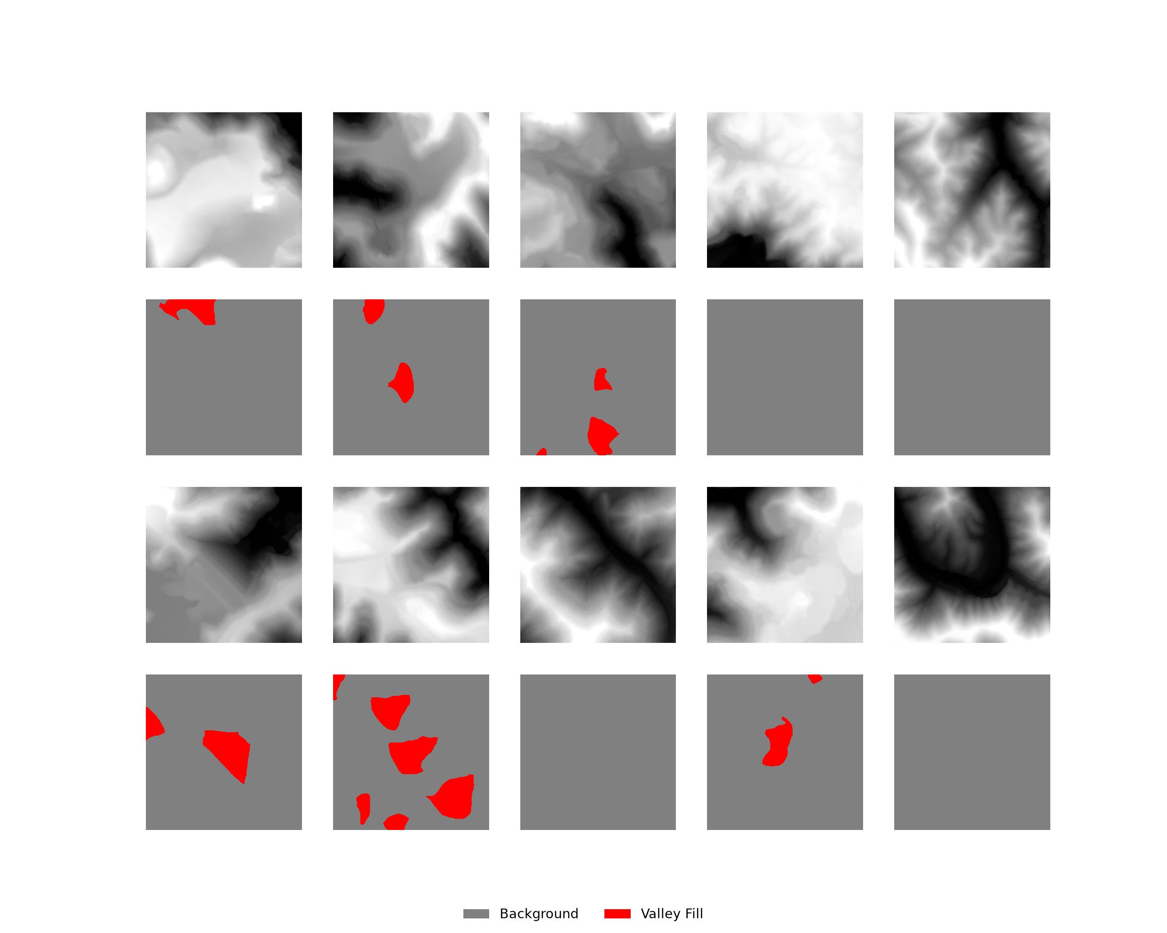
describeBatch(dynDL, nCls=2){'batchSize': 10, 'imageDataType': torch.float32, 'maskDataType': torch.int64, 'imageShape': (10, 1, 512, 512), 'maskShape': (10, 512, 512), 'bndMns': array([479.8924], dtype=float32), 'bndSDs': array([149.9514], dtype=float32), 'maskCount': array([2532246, 89194]), 'minIndex': 0, 'maxIndex': 1}Because the table stores the raster path for each chip, swapping the predictor variables, for example, replacing the DEMs with slope or hillshade raster grids, only requires changing the “imgPth” column. Similarly, a different labeling scheme can be used by changing the “maskPth” column.
20.3.5 Save Dynamic Chips
If you want to save the dynamic chips, or a subset of them, to disk, for example to inspect them in a GIS or to train a model using static chips, this can be accomplished with the saveDynamicChips() function below. It writes each chip and mask to GeoTIFF files, with the spatial reference information preserved, in “images” and “masks” subfolders, which is the same structure produced by makeChips().
To demonstrate the flexibility of dynamic chips, I save a random subset of 20 chips using a chip size of 256 cells and a cell size of 4 m. These chips cover the same 1,024 m area as the chips generated above but at a coarser spatial resolution. Generating chips with this cell size from static chips would have required resampling the DEMs and regenerating the chips. Since the saved chips use the same folder structure as static chips, they can be listed with makeChipsDF() and viewed with viewChips().
def saveDynamicChips(chipsDF, chipSize, cellSize, outDir, codeField="code", background=0):
    os.makedirs(os.path.join(outDir, "images"), exist_ok=True)
    os.makedirs(os.path.join(outDir, "masks"), exist_ok=True)
    for _, row in chipsDF.iterrows():
        out = makeDynamicChip(row, chipSize, cellSize, chipsDF.crs, codeField, background)
        profile = {"driver": "GTiff", "height": chipSize, "width": chipSize,
                   "crs": out["crs"], "transform": out["transform"]}
        name = f"chip_{row['chipID']}.tif"
        with rio.open(os.path.join(outDir, "images", name), "w", count=out["image"].shape[0],
                      dtype=out["image"].dtype, **profile) as dst:
            dst.write(out["image"])
        with rio.open(os.path.join(outDir, "masks", name), "w", count=1, dtype="uint8",
                      **profile) as dst:
            dst.write(out["mask"], 1)
dynSub = dynDF.sample(n=20, random_state=42)
saveDynamicChips(dynSub, chipSize=256, cellSize=4, outDir=outPth + "dynamicChips/")
dynChipsDF = makeChipsDF(outPth + "dynamicChips/", mode="All")
viewChips(dynChipsDF, nSamps=10, cCodes=[0, 1], cNames=["Background", "Valley Fill"],
cColors=["gray", "red"])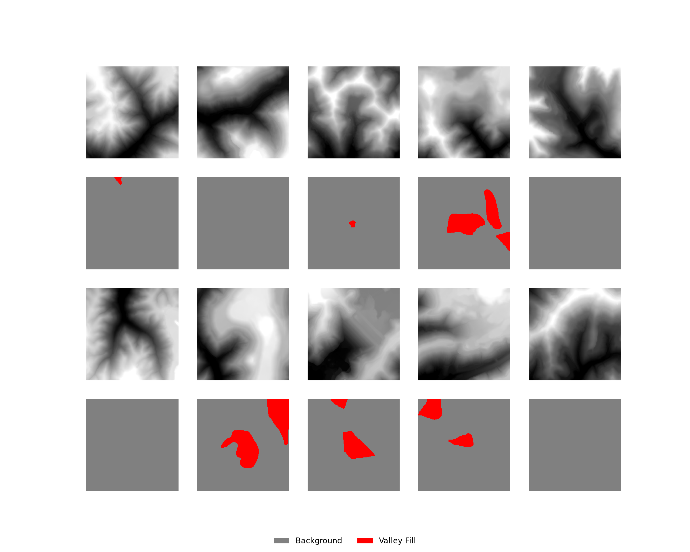
20.4 Static or Dynamic?
Which approach should you use? Here are some general guidelines:
- Static chips are simple, fast to load, and easy to inspect and share. They are a good choice when the chip size and inputs are fixed and disk space is not a concern.
- Dynamic chips are more flexible and are a good choice when experimenting with chip sizes, cell sizes, or input variables; when features are small and sparse, so that centering chips on them helps with class imbalance; or when generating and storing static chips for very large datasets is impractical.
- For assessment, it is generally best to use a consistent, systematic set of chips or to predict entire extents, as demonstrated in Chapter 19, so that the accuracy estimates are not dependent on where chips happened to be sampled. Jitter and other random augmentations should not be used for validation or testing data.
Regardless of the approach, the data should be split into training, validation, and testing partitions at the level of the raster grid, study area, or another spatial unit, as opposed to randomly assigning individual chips to partitions. Adjacent chips, and especially overlapping chips, are highly similar due to spatial autocorrelation, so assigning neighboring chips to both the training and testing partitions will result in overly optimistic accuracy estimates.
20.5 Concluding Remarks
You can now generate raster masks from vector data, generate static image chips and list them in a DataFrame, generate chips dynamically from a table of chip center locations, and load both types of chips for training using DataSets and DataLoaders. Since all of the functions are defined in this chapter, you can adapt them to your own data, for example, by changing how NoData is handled or which chips are retained. In the next chapter, we will use chips generated from the topoDL dataset to train a semantic segmentation model using the Segmentation Models package.
20.6 Questions
- Why must large geospatial raster datasets be broken into smaller image chips before they are used to train deep learning models?
- Explain the purpose of the
extentargument ofmakeMask(). Why can areas outside of the labeled extent not be assumed to be background, and how doesmakeMask()prevent them from being used as background? - What rules should be followed when assigning numeric codes to classes in a raster mask?
- Explain how the
strideXandstrideYarguments ofmakeChips()relate to thesizeargument. What are the advantages and disadvantages of generating overlapping chips? - Explain the differences between the “All”, “Positive”, and “Divided” modes of
makeChips(). Why is the “Divided” mode useful for binary problems with class imbalance? - Why were no chips written for some parts of the input image in this chapter, even when using the “All” mode? How did the dynamic chip workflow handle the same issue?
- Explain the difference between static and dynamic chips. What are the advantages and disadvantages of each?
- Why was random noise added to the valley fill centroids before they were used as chip centers? How does the
jitterargument ofDynamicSegDatasetextend this idea, and why was a negativeextentCropvalue used?