import numpy as np
import pandas as pd
import matplotlib.pyplot as plt
import rasterio as rio
from rasterio import features
from rasterio.windows import from_bounds
import geopandas as gpd
from shapely.geometry import shape, box
from shapely.ops import unary_union

import torch
import torch.nn as nn
from torch.utils.data import Dataset, DataLoader
import torchvision
from torchvision.models.detection import maskrcnn_resnet50_fpn_v2
from torchvision.models.detection.faster_rcnn import FastRCNNPredictor
from torchvision.models.detection.mask_rcnn import MaskRCNNPredictor
from torchvision.utils import draw_bounding_boxes, draw_segmentation_masks
from torchmetrics.detection import MeanAveragePrecision
import albumentations as A
import lightning as L
from lightning.pytorch.callbacks import ModelCheckpoint
from lightning.pytorch.loggers import CSVLogger
from terrainseg import lspModule

device = torch.device("cuda:0" if torch.cuda.is_available() else "cpu")23 Instance Segmentation with Mask R-CNN
23.1 Introduction
In Chapter 22, we performed instance segmentation using a segmentation-based method, UNet-ID, which modifies a semantic segmentation architecture and separates objects in a post-processing step. In this chapter, we explore a detection-based method: Mask R-CNN (He et al., 2017). Mask R-CNN extends the Faster R-CNN object detection architecture (Ren et al., 2015). Object detection models predict a bounding box, a class label, and a confidence score for each object. Mask R-CNN adds a branch that predicts a binary mask for each detected object. Since each object is detected separately, instances are produced directly, without post-processing to separate touching objects.
He, K., Gkioxari, G., Dollár, P. and Girshick, R., 2017. “Mask R-CNN.” In Proceedings of the IEEE International Conference on Computer Vision (pp. 2961-2969).
Ren, S., He, K., Girshick, R. and Sun, J., 2015. “Faster R-CNN: Towards real-time object detection with region proposal networks.” Advances in Neural Information Processing Systems, 28.
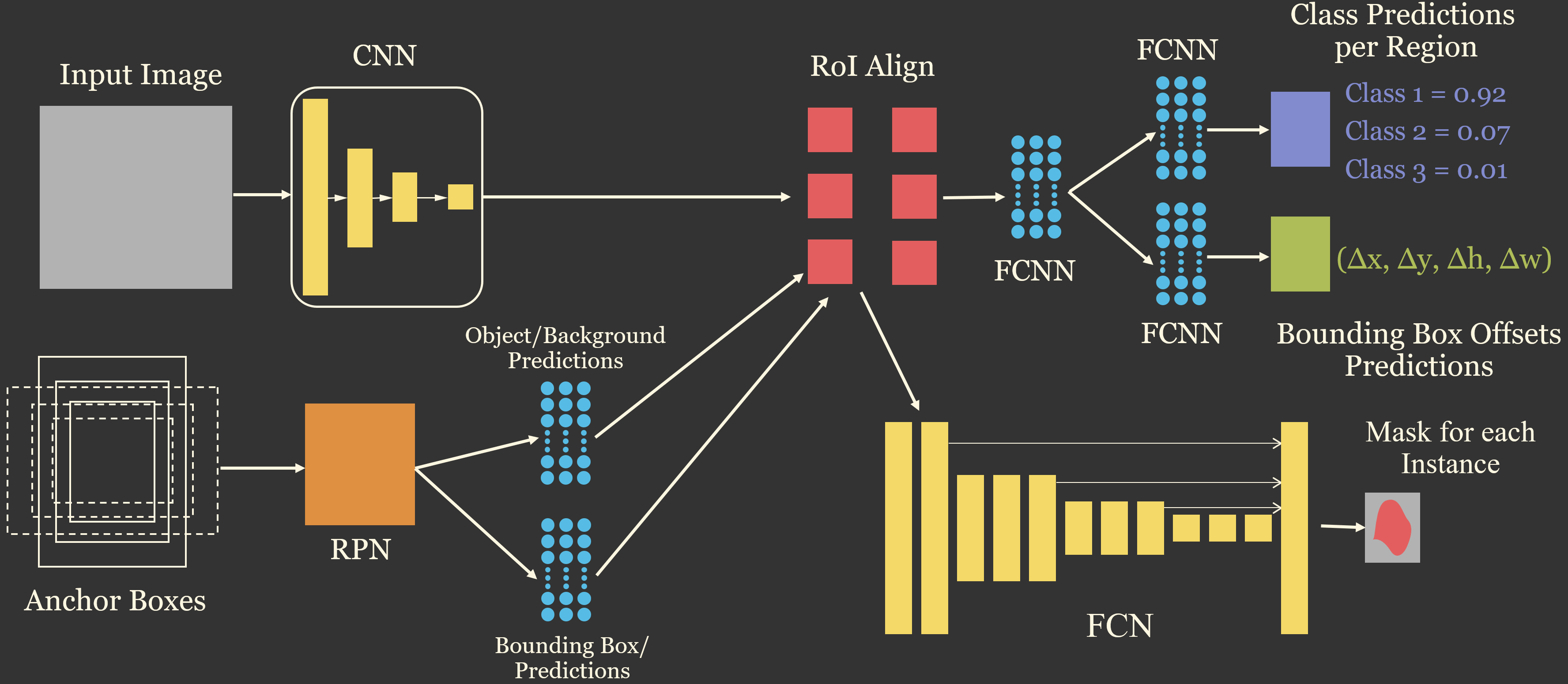
Mask R-CNN is a two-stage detector. Its components are:
- Backbone with a feature pyramid network (FPN): a CNN, such as ResNet-50, extracts feature maps at several resolutions. The FPN combines them using a top-down pathway with lateral connections, similar in spirit to the skip connections in UNet, so that feature maps at every resolution contain both detailed and semantically meaningful information. This allows objects of very different sizes to be detected.
- Region proposal network (RPN): at each location on the feature maps, a set of anchor boxes with different sizes and aspect ratios is defined. The RPN predicts whether each anchor contains an object and how the anchor should be adjusted to better fit the object. The highest-scoring adjusted anchors, after removing duplicates using non-maximum suppression, are the region proposals.
- RoIAlign: the features within each proposal are extracted from the feature maps and resampled to a fixed size (e.g., 7x7 for the box branch and 14x14 for the mask branch) using bilinear interpolation. RoIAlign avoids the rounding of coordinates used in earlier methods, which is important for producing accurate masks.
- Box head: for each proposal, fully connected layers predict the class and refine the bounding box.
- Mask head: for each proposal, a small fully convolutional network predicts a mask (28x28 by default) for each class. Only the mask for the predicted class is used, and it is resized to fit the predicted bounding box.
These components are conceptualized in Figure 23.1.
The loss is the sum of several components: the RPN’s object and box regression losses and the second stage’s classification, box regression, and mask losses. Fortunately, torchvision provides a complete implementation of Mask R-CNN, including pre-trained weights from the COCO dataset, and it calculates these losses internally. Our task is to prepare the data in the expected format, adapt the model to our classes and data, train it, and assess the results.
The example in this chapter maps individual valley fill faces, the engineered slopes created when mining spoil is placed in valleys adjacent to mountaintop removal coal mines, using data derived from the vfillDL dataset introduced in Chapter 20. This is the same dataset used for UNet-ID in Chapter 22, so the results of the two approaches can be compared.
23.2 The Valley Fill Instance Dataset
The vfillDL dataset provides lidar-derived digital terrain models (DTMs) with a 2 m cell size and polygons of the valley fill faces for several study areas in West Virginia, Kentucky, and Virginia. To keep the example manageable, I only use three of the study areas: KY1 for training, KY2 for validation, and VA1 for testing. Since the three areas are geographically separated, the validation and test data provide an assessment of how well the model generalizes to new areas. This is a fairly small training set: KY1 contains 553 valley fill faces. Adding the larger West Virginia training area would likely improve the results, so the model trained here should not be considered optimal.
I created the image chips and instance masks ahead of time; the resulting dataset, vfillInst, is provided as a separate download (see Table 2). The DTM and polygons for VA1, which are used to map a larger area at the end of the chapter, are part of the vfillDL dataset. Each chip is 512x512 cells and contains three land surface parameters (LSPs) calculated from the DTM using the lspModule class from the terrainseg package: a hillslope-scale topographic position index (TPI), the square root of slope, and a multidirectional hillshade. All three are already scaled from 0 to 1. The LSPs were calculated for 640x640 cell windows, and 64 cells were trimmed from each side, since the convolutions used to calculate the LSPs pad the edges of the input with zeros and produce incorrect values near the edges. The radii that define the moving windows used by lspModule are specified as numbers of cells, as opposed to map units. The default radii were designed for data with a 1 m cell size, so I halved them for these 2 m data; otherwise, the windows would cover twice the intended distance, and roughly 20% of the TPI values would be clipped at the ±10 m limits used to rescale the TPI. I use the same settings when predicting to new areas below.
Each mask chip is an instance raster: background cells are coded as 0, and the cells within each valley fill face are coded using a unique integer ID. The masks were created by rasterizing the polygons, so each polygon is a separate instance. The chips were generated as follows:
- Training: one chip centered on each valley fill face in KY1. All valley fill faces that fall within a chip are included in its mask, so a face can occur in several overlapping chips. Centering the chips on the objects guarantees that every valley fill face is fully contained in at least one chip.
- Validation and testing: a grid of non-overlapping chips covering KY2 and VA1. Chips centered on the objects would make the assessment overly optimistic, since in practice the model must be applied to the entire landscape.
- Background: chips that contain no valley fill faces were sampled from the grid in each area, with one background chip for every two chips containing valley fill faces. These help the model learn to avoid false positives on the mine benches, roads, and other features that resemble valley fill faces.
Each partition is described by a CSV file that lists the chip names, whether the chip contains valley fill faces (“Positive”) or not (“Background”), and the number of instances.
ImportantData Location
This chapter uses the vfillInst dataset, which is provided as a separate download (vfillInst.zip) in the download menu in the sidebar, and the VA1 DTM and polygons from the vfillDL dataset, which is too large to include in the book download and must be downloaded from the source listed in Table 2. By default, the code expects the uncompressed vfillInst and vfillDL folders to be saved in the data/files folder (data/files/vfillInst and data/files/vfillDL). If you saved the data elsewhere, set folder below and dtmPath and the reference polygon path in the section on predicting to geospatial data to the correct locations on your machine.
# Set this to the location of the uncompressed vfillInst folder on your machine.
folder = "data/files/vfillInst/"
trainDF = pd.read_csv(folder + "trainDF.csv")
valDF = pd.read_csv(folder + "valDF.csv")
testDF = pd.read_csv(folder + "testDF.csv")

pd.DataFrame({split: [len(df), (df["division"] == "Positive").sum(), df["nInst"].sum()]
              for split, df in zip(["train", "val", "test"], [trainDF, valDF, testDF])},
             index=["Chips", "Positive chips", "Instances"])
train val test
Chips 795 180 193
Positive chips 533 119 127
Instances 1574 214 19123.3 Preparing the Data
23.3.1 Target Format
The torchvision detection models expect the data in a different format than the semantic segmentation models used so far. Each image is a float tensor with a shape of (C, H, W); the model normalizes the images internally. Each image’s labels are provided as a dictionary, called the target, with the following keys:
-
"boxes": a float tensor with a shape of (N, 4), where N is the number of objects in the image, giving each object’s bounding box as (xmin, ymin, xmax, ymax) in pixel coordinates. -
"labels": a long integer tensor with a shape of (N), giving each object’s class. Class 0 is reserved for the background, so the object classes are coded starting at 1. -
"masks": a uint8 tensor with a shape of (N, H, W), giving a binary mask for each object.
Since the number of objects differs between images, the images in a mini-batch cannot be stacked into a single tensor. Instead, the model accepts a list of image tensors and a list of target dictionaries. Images do not even need to have the same size.
23.3.2 Instances from an Instance Raster
The function below converts an instance chip to a target dictionary. For each object, it extracts the binary mask and calculates the bounding box from the extent of the mask. Since there is only one class, all labels are 1. Objects smaller than minPix cells are removed. In this dataset, these are mostly small slivers of valley fill faces cut by the edge of a chip, which are difficult to detect and can destabilize training. I use 200 cells (800 m2), which removes roughly 5% of the training instances; the median instance is roughly 4,600 cells. Images with no objects are allowed: in this case, the boxes tensor must have a shape of (0, 4) as opposed to being empty.
def instToTarget(inst, minPix=200):
    ids = [i for i in np.unique(inst) if i != 0]
    masks, boxes = [], []
    for i in ids:
        m = inst == i
        if m.sum() < minPix:
            continue
        ys, xs = np.where(m)
        masks.append(m)
        boxes.append([xs.min(), ys.min(), xs.max() + 1, ys.max() + 1])
    H, W = inst.shape
    return {
        "boxes": torch.tensor(boxes, dtype=torch.float32).reshape(-1, 4),
        "labels": torch.ones(len(boxes), dtype=torch.int64),
        "masks": torch.from_numpy(np.stack(masks)).to(torch.uint8) if masks
                 else torch.zeros((0, H, W), dtype=torch.uint8),
    }
23.3.3 DataSet and Collate Function
The DataSet reads each image chip and instance chip, applies transforms, and returns the image tensor and the target dictionary. Albumentations is applied to the image and the instance chip together, using the mask argument, so that geometric transformations are applied consistently; the target is then derived from the transformed instance chip. Deriving the boxes from the transformed masks, as opposed to transforming the boxes directly, ensures that the boxes always fit the objects, even after rotations. I only use flips and 90-degree rotations. Brightness and contrast adjustments, which are common for photographs, are not appropriate here, since the LSP values have physical meanings.
Since the default DataLoader behavior is to stack the items in a mini-batch into tensors, which is not possible for the targets, a collate function that returns the images and targets as tuples is provided to the DataLoader.
class InstanceDataset(Dataset):
    def __init__(self, df, folder, split, transform=None, minPix=200):
        self.df = df
        self.folder = folder
        self.split = split
        self.transform = transform
        self.minPix = minPix

    def __getitem__(self, idx):
        chpN = self.df.iloc[idx]["chpN"]
        with rio.open(f"{self.folder}{self.split}/images/{chpN}") as src:
            image = np.transpose(src.read().astype("float32"), (1, 2, 0))
        with rio.open(f"{self.folder}{self.split}/masks/{chpN}") as src:
            inst = src.read(1).astype("int32")
        if self.transform is not None:
            out = self.transform(image=image, mask=inst)
            image, inst = out["image"], out["mask"]
        image = torch.from_numpy(np.ascontiguousarray(np.transpose(image, (2, 0, 1))))
        return image, instToTarget(inst, self.minPix)

    def __len__(self):
        return len(self.df)

def collate_fn(batch):
    return tuple(zip(*batch))
trainTransform = A.Compose([A.HorizontalFlip(p=0.5), A.VerticalFlip(p=0.5), A.RandomRotate90(p=0.5)])
trainDS = InstanceDataset(trainDF, folder, "train", trainTransform)
valDS = InstanceDataset(valDF, folder, "val")
testDS = InstanceDataset(testDF, folder, "test")
trainDL = DataLoader(trainDS, batch_size=4, shuffle=True, collate_fn=collate_fn, num_workers=0)
valDL = DataLoader(valDS, batch_size=4, shuffle=False, collate_fn=collate_fn, num_workers=0)
testDL = DataLoader(testDS, batch_size=4, shuffle=False, collate_fn=collate_fn, num_workers=0)
torch.manual_seed(42)
images, targets = next(iter(trainDL))
print(len(images), images[0].shape, targets[0]["boxes"].shape, targets[0]["masks"].shape)4 torch.Size([3, 512, 512]) torch.Size([2, 4]) torch.Size([2, 512, 512])To check the data, I plot the images with their bounding boxes and masks using torchvision’s drawing utilities, which expect an 8-bit RGB image tensor. The toRGB8() function converts the hillshade band to an 8-bit, three-band image after applying a linear stretch.
def toRGB8(image, band=2):
    hs = image[band]
    lo, hi = torch.quantile(hs, 0.01), torch.quantile(hs, 0.99)
    hs = ((hs - lo) / (hi - lo + 1e-6)).clamp(0, 1)
    return (hs * 255).to(torch.uint8).repeat(3, 1, 1)

def drawInstances(image, masks, boxes, color="yellow"):
    viz = toRGB8(image)
    if len(masks) > 0:
        viz = draw_segmentation_masks(viz, masks.bool(), alpha=0.4, colors=color)
        viz = draw_bounding_boxes(viz, boxes, colors=color, width=2)
    return viz.permute(1, 2, 0)

fig, axs = plt.subplots(1, 4, figsize=(16, 4))
for i, ax in enumerate(axs):
    ax.imshow(drawInstances(images[i], targets[i]["masks"], targets[i]["boxes"]))
    ax.set_title(f"{len(targets[i]['boxes'])} instances")
    ax.axis("off")
plt.show()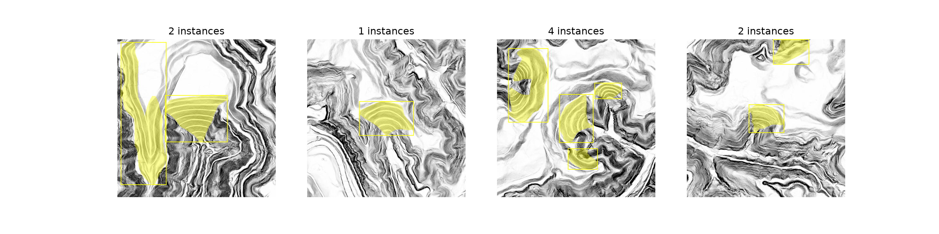
23.4 Defining the Model
torchvision provides two versions of Mask R-CNN with a ResNet-50 FPN backbone. I use the improved version, maskrcnn_resnet50_fpn_v2(), which was trained with a more modern training recipe and generally performs better. The model is initialized with weights pre-trained on the COCO dataset, which contains 91 categories of everyday objects. To adapt the model to our problem, the box predictor and mask predictor must be replaced so that they output the correct number of classes. The number of classes includes the background, so for a single class, such as valley fill faces, nCls is 2.
Several other settings are worth adjusting for geospatial data:
-
min_sizeandmax_size: by default, torchvision resizes each image so that its shorter side is 800 pixels, which is appropriate for photographs but would greatly enlarge 512x512 image chips and increase memory use and training time. Settingmin_sizeandmax_sizeto the chip size avoids resizing. -
image_meanandimage_std: the values used to normalize the images inside the model. The defaults are the ImageNet RGB means and standard deviations, which are not appropriate for our LSPs, so I calculate the mean and standard deviation of each band from the training chips. -
trainable_backbone_layers: by default, torchvision freezes the earliest stages of the pre-trained backbone and only trains the last three of the five stages. Since our LSPs are very different from the COCO photographs, I train all five stages. -
box_detections_per_img: the maximum number of objects returned for each image, 100 by default. This is plenty for valley fill faces, but it may need to be increased for dense objects, such as buildings in urban areas.
bandSum, bandSqSum, nCells = np.zeros(3), np.zeros(3), 0
for chpN in trainDF["chpN"]:
    with rio.open(f"{folder}train/images/{chpN}") as src:
        x = src.read().reshape(3, -1).astype("float64")
    bandSum += x.sum(axis=1)
    bandSqSum += (x ** 2).sum(axis=1)
    nCells += x.shape[1]
bandMeans = bandSum / nCells
bandSDs = np.sqrt(bandSqSum / nCells - bandMeans ** 2)
bandMeans, bandSDs = [round(float(v), 4) for v in bandMeans], [round(float(v), 4) for v in bandSDs]
print(bandMeans, bandSDs)
[0.5004, 0.4202, 0.6488] [0.1587, 0.1596, 0.0541]def makeMaskRCNN(nCls, bandMeans, bandSDs, chipSize=512, weights="DEFAULT", trainableLayers=5):
# trainable_backbone_layers only applies when pre-trained weights are loaded
model = maskrcnn_resnet50_fpn_v2(weights=weights, min_size=chipSize, max_size=chipSize,
image_mean=bandMeans, image_std=bandSDs,
trainable_backbone_layers=trainableLayers if weights else None)
inFeat = model.roi_heads.box_predictor.cls_score.in_features
model.roi_heads.box_predictor = FastRCNNPredictor(inFeat, nCls)
inFeatMask = model.roi_heads.mask_predictor.conv5_mask.in_channels
model.roi_heads.mask_predictor = MaskRCNNPredictor(inFeatMask, 256, nCls)
return model
model = makeMaskRCNN(2, bandMeans, bandSDs)23.4.1 More Than Three Bands
The pre-trained backbone expects three input bands, which is why I use three of the LSPs. To use more bands, such as the six LSPs that lspModule can generate or multispectral imagery, the first convolutional layer of the backbone is replaced, as we did for classification in Chapter 12, and the normalization values must have one value per band. Since the replaced layer is randomly initialized, one common strategy is to copy the pre-trained weights into the first three input channels and initialize the additional channels with the mean of the pre-trained weights, which preserves much of the benefit of pre-training. This function is not used in the remainder of the chapter.
def adaptInputChannels(model, nChn, bandMeans, bandSDs):
    old = model.backbone.body.conv1
    new = nn.Conv2d(nChn, old.out_channels, kernel_size=7, stride=2, padding=3, bias=False)
    with torch.no_grad():
        new.weight[:, :3] = old.weight
        if nChn > 3:
            new.weight[:, 3:] = old.weight.mean(dim=1, keepdim=True)
    model.backbone.body.conv1 = new
    model.transform.image_mean = list(bandMeans)
    model.transform.image_std = list(bandSDs)
    return model
23.4.2 Training and Inference Modes
The torchvision detection models behave differently in training and evaluation modes. In training mode, the model must be given both the images and the targets, and it returns a dictionary of the loss components. In evaluation mode, the model is given only the images, and it returns a list containing a dictionary of predictions for each image, with the keys "boxes", "labels", "scores", and "masks". The predicted masks are probabilities with a shape of (N, 1, H, W), which are generally thresholded at 0.5. Since the new predictors have not been trained yet, the untrained model’s predictions are not meaningful.
model = model.to(device)
imagesD = [im.to(device) for im in images]
targetsD = [{k: v.to(device) for k, v in t.items()} for t in targets]

model.train()
lossDict = model(imagesD, targetsD)
print({k: round(v.item(), 4) for k, v in lossDict.items()})
{'loss_classifier': 0.6161, 'loss_box_reg': 0.1151, 'loss_mask': 1.4037, 'loss_objectness': 0.2296, 'loss_rpn_box_reg': 0.0148}model.eval()
with torch.no_grad():
preds = model(imagesD)
print(preds[0].keys(), preds[0]["masks"].shape)dict_keys(['boxes', 'labels', 'scores', 'masks']) torch.Size([100, 1, 512, 512])23.5 Training with Lightning
Since Mask R-CNN calculates its own losses, the LightningModule’s training_step() passes the images and targets to the model and sums the returned loss components. Each component is also logged, which is useful for diagnosing training problems; for example, a high mask loss but a low box loss indicates that objects are being detected but their shapes are not being captured well.
Validation requires care. In evaluation mode, the model returns predictions as opposed to losses, so I use the validation data to calculate mean average precision (mAP), described below, using torchmetrics’ MeanAveragePrecision metric. Note that MeanAveragePrecision requires the pycocotools package (or faster-coco-eval) to be installed. Setting iou_type=["bbox", "segm"] calculates the metric for both the bounding boxes and the masks. The predicted mask probabilities are thresholded and converted to boolean tensors before being passed to the metric.
class LitMaskRCNN(L.LightningModule):
    def __init__(self, model, lr=1e-4, weightDecay=1e-4):
        super().__init__()
        self.save_hyperparameters(ignore=["model"])
        self.model = model
        self.lr = lr
        self.weightDecay = weightDecay
        self.valMAP = MeanAveragePrecision(iou_type=["bbox", "segm"])

    def forward(self, images):
        return self.model(images)

    def training_step(self, batch, batch_idx):
        images, targets = batch
        lossDict = self.model(list(images), list(targets))
        loss = sum(lossDict.values())
        bs = len(images)
        self.log("train_loss", loss, on_step=False, on_epoch=True, prog_bar=True, batch_size=bs)
        self.log_dict({f"train_{k}": v for k, v in lossDict.items()},
                      on_step=False, on_epoch=True, batch_size=bs)
        return loss

    def validation_step(self, batch, batch_idx):
        images, targets = batch
        preds = self.model(list(images))
        for p in preds:
            p["masks"] = p["masks"].squeeze(1) > 0.5
        tgts = [{"boxes": t["boxes"], "labels": t["labels"], "masks": t["masks"].bool()} for t in targets]
        self.valMAP.update(preds, tgts)

    def on_validation_epoch_end(self):
        res = self.valMAP.compute()
        self.log_dict({"val_segm_map": res["segm_map"], "val_segm_map_50": res["segm_map_50"],
                       "val_bbox_map": res["bbox_map"], "val_bbox_map_50": res["bbox_map_50"]},
                      prog_bar=True)
        self.valMAP.reset()

    def configure_optimizers(self):
        params = [p for p in self.model.parameters() if p.requires_grad]
        optimizer = torch.optim.AdamW(params, lr=self.lr, weight_decay=self.weightDecay)
        scheduler = torch.optim.lr_scheduler.CosineAnnealingLR(optimizer, T_max=self.trainer.max_epochs)
        return {"optimizer": optimizer, "lr_scheduler": {"scheduler": scheduler, "interval": "epoch"}}
I train the model for 30 epochs with a mini-batch size of 4, using the AdamW optimizer with a learning rate of 1e-4 that is decreased using cosine annealing, gradient clipping, and bfloat16 mixed precision. The checkpoint with the highest validation mask mAP is retained. After training, I save the state dictionary of the best model, which is smaller than the checkpoint since it does not include the optimizer state.
L.seed_everything(42)
litModel = LitMaskRCNN(makeMaskRCNN(2, bandMeans, bandSDs), lr=1e-4)
ckpt = ModelCheckpoint(dirpath="data/output/maskrcnnVfill/", filename="best",
                       monitor="val_segm_map", mode="max")
trainer = L.Trainer(max_epochs=30, accelerator="gpu", devices=1, precision="bf16-mixed",
                    gradient_clip_val=5.0, callbacks=[ckpt],
                    logger=CSVLogger("data/output/", name="maskrcnnVfill"))
trainer.fit(litModel, train_dataloaders=trainDL, val_dataloaders=valDL)

best = LitMaskRCNN.load_from_checkpoint(ckpt.best_model_path,
                                        model=makeMaskRCNN(2, bandMeans, bandSDs, weights=None))
torch.save(best.model.state_dict(), "data/output/maskrcnnVfill.pt")
Training took about 39 minutes on my machine with a single GPU. If you do not want to or cannot train the model, the saved state dictionary and training log have been provided with the text. The training loss components and the validation mAP are plotted below. All of the training losses decrease throughout training, with the mask loss remaining the largest. In contrast, the validation mask mAP reaches its highest value, 0.455, at epoch 10 (counting from 0) and then levels off at roughly 0.43, while the validation mask AP50 remains at roughly 0.70. The continued decrease in the training loss without a corresponding improvement for the validation data suggests that the model is overfitting to the small training set. Since the checkpoint with the highest validation mask mAP was retained, the saved model is from epoch 10.
resultsDF = pd.read_csv("data/models/maskrcnnVfillLogs.csv")
trainRes = resultsDF.dropna(subset=["train_loss"])
valRes = resultsDF.dropna(subset=["val_segm_map"])

fig, axs = plt.subplots(1, 2, figsize=(12, 4))
trainRes.plot(x="epoch", y=["train_loss_classifier", "train_loss_box_reg", "train_loss_mask",
                            "train_loss_objectness", "train_loss_rpn_box_reg"], ax=axs[0],
              title="Training loss components")
valRes.plot(x="epoch", y=["val_bbox_map", "val_segm_map", "val_bbox_map_50", "val_segm_map_50"],
            ax=axs[1], title="Validation mAP")
plt.show()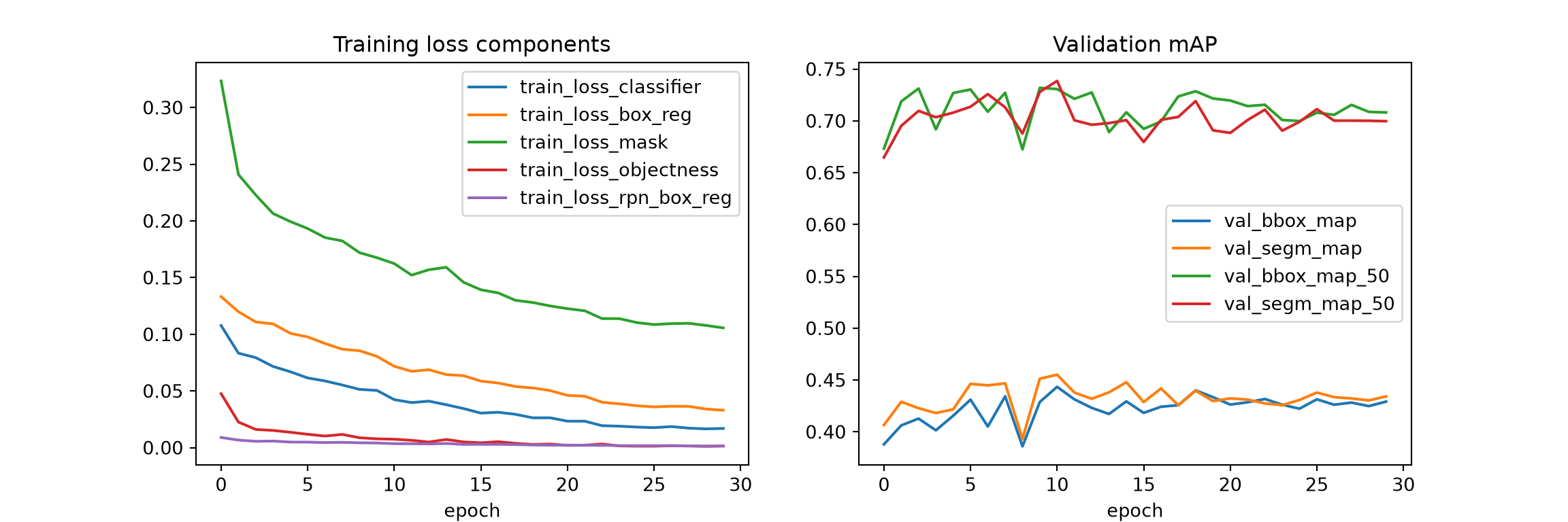
A few notes about training Mask R-CNN:
- Mask R-CNN is memory intensive, so small mini-batches, such as 2 to 8 images, are common. Batch normalization statistics are unreliable when calculated from very small mini-batches. For this reason, detection models generally use “frozen” batch normalization in the pre-trained backbone, in which the statistics and parameters learned during pre-training are fixed. When pre-trained weights are used, torchvision’s Mask R-CNN models replace the backbone’s batch normalization layers with
FrozenBatchNorm2dlayers. Gradient accumulation (Chapter 8) can be used to increase the effective mini-batch size. - Gradient clipping is helpful for stabilizing training, especially early on.
- Mixed precision can be used, but the detection losses can be sensitive to reduced precision. If training is unstable, try 32-bit precision.
23.6 Assessment
23.6.1 Mean Average Precision
Object detection and instance segmentation models are commonly assessed using average precision (AP). Each predicted object has a confidence score. For a given IoU threshold, predictions are sorted by score, each is matched to a reference object if their IoU exceeds the threshold (as in Chapter 22), and precision and recall are calculated as the score threshold is lowered. AP summarizes the resulting precision-recall curve as a single value, similar to the area under the precision-recall curve discussed in Chapter 4. Several versions are commonly reported:
- AP50 (or mAP@0.5): AP with an IoU threshold of 0.5, which counts a prediction as correct if it overlaps a reference object reasonably well.
- AP75: AP with a stricter IoU threshold of 0.75, which requires more precise boxes or masks.
- mAP (or AP@[0.5:0.95]): the mean of AP calculated at IoU thresholds from 0.5 to 0.95 in steps of 0.05. This is the primary metric used by the COCO benchmark, and it rewards precise localization.
- AP for small, medium, and large objects, defined by their area in pixels. These are useful when object sizes vary greatly.
When there are multiple classes, AP is calculated for each class and averaged, which is why it is called mean average precision. Mask-based AP ("segm") is generally lower than box-based AP ("bbox") since masks must match the objects’ shapes as opposed to only their extents.
To assess the model, I load the saved state dictionary into a new model and predict the VA1 test chips. The predictions and targets are retained so that they can also be used to calculate the object-level metrics below.
model = makeMaskRCNN(2, bandMeans, bandSDs, weights=None)
model.load_state_dict(torch.load("data/models/maskrcnnVfill.pt", map_location=device))
model = model.to(device).eval()

testMAP = MeanAveragePrecision(iou_type=["bbox", "segm"])
allPreds, allTargets = [], []
with torch.no_grad():
    for images, targets in testDL:
        preds = model([im.to(device) for im in images])
        preds = [{k: v.cpu() for k, v in p.items()} for p in preds]
        for p in preds:
            p["masks"] = p["masks"].squeeze(1) > 0.5
        targets = [{**t, "masks": t["masks"].bool()} for t in targets]
        testMAP.update(preds, targets)
        allPreds += preds
        allTargets += targets
results = testMAP.compute()

metricNames = ["map", "map_50", "map_75", "map_small", "map_medium", "map_large"]
pd.DataFrame({"Boxes": [round(float(results[f"bbox_{m}"]), 3) for m in metricNames],
              "Masks": [round(float(results[f"segm_{m}"]), 3) for m in metricNames]},
             index=["mAP", "AP50", "AP75", "AP small", "AP medium", "AP large"])
Boxes Masks
mAP 0.254 0.255
AP50 0.466 0.446
AP75 0.251 0.283
AP small 0.220 0.157
AP medium 0.312 0.309
AP large 0.157 0.202The results for the VA1 test data are substantially lower than those for the KY2 validation data: the mask mAP is 0.255, and the mask AP50 is 0.446, compared to 0.455 and 0.739 for the validation data. Since the model was selected using KY2, the validation results are somewhat optimistic; however, the size of the difference suggests that the valley fill faces and the surrounding terrain in VA1 differ from those in the two Kentucky study areas, and that the model, trained using a single study area, does not generalize well to new areas. Training with data from more areas, such as the West Virginia training area, would likely help. The mask and box metrics are similar, and the mask AP75 is slightly higher than the box AP75, which suggests that, when a valley fill face is detected, its shape is captured about as well as its extent.
23.6.2 Object-Level Precision, Recall, and F1-Score
Since mAP integrates over all confidence scores, it does not depend on a specific score threshold. However, to produce a map, a threshold must be selected, and predictions with lower scores are discarded. The objectMetrics() function calculates the object-level precision, recall, and F1-score, as used for UNet-ID in Chapter 22, for a given score threshold. Predicted and reference objects are matched if the IoU of their masks is greater than 0.5. Since two objects that do not overlap each other cannot both have an IoU greater than 0.5 with the same object, each prediction can be matched to at most one reference object. Matched predictions are true positives, unmatched predictions are false positives, and unmatched reference objects are false negatives.
def maskIoU(a, b):
    a, b = a.flatten(1).float(), b.flatten(1).float()
    inter = a @ b.T
    union = a.sum(1)[:, None] + b.sum(1)[None, :] - inter
    return inter / union.clamp(min=1)

def objectMetrics(preds, targets, scoreThresh=0.5, iouThresh=0.5):
    tp, nPred, nRef = 0, 0, 0
    for p, t in zip(preds, targets):
        pm = p["masks"][p["scores"] >= scoreThresh]
        tm = t["masks"]
        nPred += len(pm)
        nRef += len(tm)
        if len(pm) > 0 and len(tm) > 0:
            tp += int((maskIoU(pm, tm).max(dim=0).values > iouThresh).sum())
    precision = tp / max(nPred, 1)
    recall = tp / max(nRef, 1)
    f1 = 2 * precision * recall / max(precision + recall, 1e-6)
    return {"Precision": round(precision, 3), "Recall": round(recall, 3), "F1": round(f1, 3)}

pd.DataFrame({s: objectMetrics(allPreds, allTargets, s) for s in [0.3, 0.5, 0.7, 0.9]}).T
Precision Recall F1
0.3 0.359 0.562 0.438
0.5 0.475 0.508 0.491
0.7 0.565 0.449 0.500
0.9 0.719 0.373 0.491As the score threshold increases, precision increases and recall decreases, since fewer predictions are kept. The F1-score is roughly 0.49 to 0.50 for thresholds from 0.5 to 0.9, so I use a threshold of 0.5 below, which balances precision (0.475) and recall (0.508). Note that the test chips are a grid, so many valley fill faces are cut by the chip edges. Partial objects are harder to detect and to match, so these chip-based metrics are lower than they would be if each object were predicted in its entirety, as is the case when mapping a larger area as described below.
To visualize the results, I plot the reference objects (left) and the predictions with a score of at least 0.5 (right) for several test chips.
showIdx = testDF.index[testDF["nInst"] >= 2][[0, 5, 10, 15]]
fig, axs = plt.subplots(2, 4, figsize=(16, 8))
for j, i in enumerate(showIdx):
    image = testDS[i][0]
    t, p = allTargets[i], allPreds[i]
    keep = p["scores"] >= 0.5
    axs[0, j].imshow(drawInstances(image, t["masks"], t["boxes"], "yellow"))
    axs[0, j].set_title(f"Reference: {len(t['boxes'])}")
    axs[1, j].imshow(drawInstances(image, p["masks"][keep], p["boxes"][keep], "cyan"))
    axs[1, j].set_title(f"Predicted: {int(keep.sum())}")
for ax in axs.flat:
    ax.axis("off")
plt.show()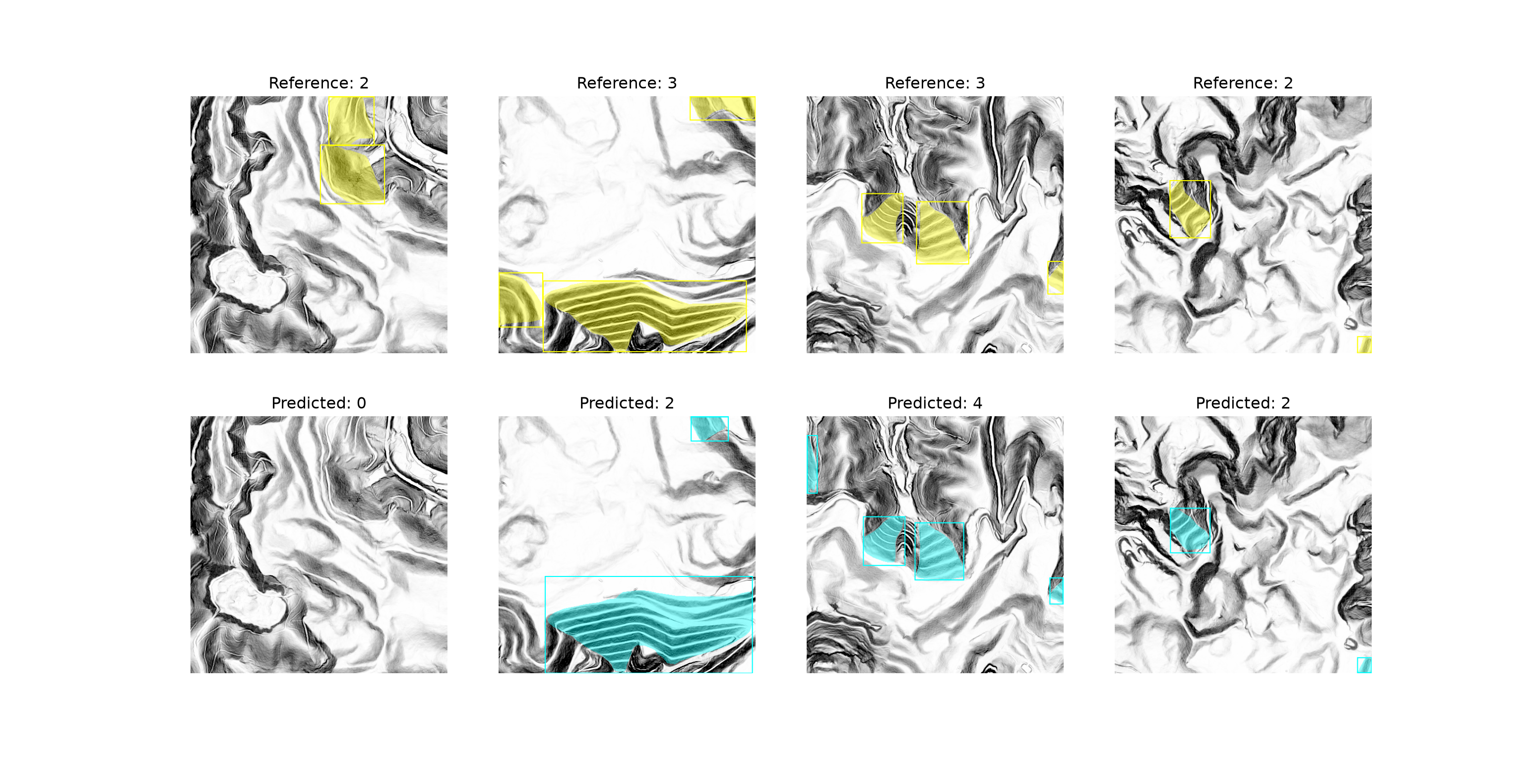
23.7 Predicting to Geospatial Data
To produce a map, the predictions must be generated for an entire area and converted to polygons in map coordinates. The predictDTM() function below performs the following steps for a rectangular area within a DTM:
- The DTM is read for the area plus a 64-cell buffer, and the LSPs are calculated using
lspModulewith the same settings used to create the chips. The buffer is then removed, which avoids the edge effects described above. Calculating the LSPs once for the entire area, as opposed to separately for each chip, avoids recalculating the overlapping portions. - The LSP stack is processed as overlapping 512x512 chips. The
stridecontrols the spacing of the chips; with a stride of 384, adjacent chips overlap by 128 cells. - The predictions with a score above a threshold are kept, and each mask is thresholded and converted to a polygon using
rasterio.features.shapes()with the chip’s transform. If a mask consists of several separate regions, they are combined into a single multipolygon.
Unlike semantic segmentation, where overlapping predictions can be cropped and mosaicked, the same object may be detected in several overlapping chips, sometimes as a complete object and sometimes as only the portion within the chip. Duplicate detections are removed in two ways. First, each chip is only responsible for the objects whose bounding box center falls within its central portion, the region extending half of the overlap from each internal edge, so each location is the responsibility of exactly one chip. Second, non-maximum suppression (torchvision.ops.nms()) is applied to the boxes from all chips in map coordinates to remove any remaining duplicates.
lspM = lspModule(cell_size=2.0, spat_dim=640, inner_radius=1, outer_radius=5,
                 hs_radius=25, smooth_radius=6).to(device).eval()

def predictDTM(model, lspM, dtmPath, bounds, chipSize=512, stride=384, pad=64,
               scoreThresh=0.5, maskThresh=0.5, nmsIoU=0.3):
    with rio.open(dtmPath) as src:
        win = from_bounds(*bounds, transform=src.transform).round_offsets().round_lengths()
        r0, c0, H, W = int(win.row_off), int(win.col_off), int(win.height), int(win.width)
        dtm = src.read(1, window=((r0 - pad, r0 + H + pad), (c0 - pad, c0 + W + pad)))
        areaTransform = src.window_transform(win)
        crs = src.crs

    with torch.no_grad():
        lsps = lspM(torch.from_numpy(dtm).float()[None, None].to(device))
    lsps = lsps[0, [0, 1, 3], pad:-pad, pad:-pad]       # tpiHS, slp, hillshade

    def starts(n):
        s = list(range(0, n - chipSize + 1, stride))
        return s if s[-1] == n - chipSize else s + [n - chipSize]

    margin = (chipSize - stride) // 2
    rows, mapBoxes = [], []
    rowStarts, colStarts = starts(H), starts(W)
    for r in rowStarts:
        for c in colStarts:
            with torch.no_grad():
                pred = model([lsps[:, r:r + chipSize, c:c + chipSize]])[0]
            # Central region this chip is responsible for (full extent at the area's edges)
            yMin = 0 if r == rowStarts[0] else margin
            yMax = chipSize if r == rowStarts[-1] else chipSize - margin
            xMin = 0 if c == colStarts[0] else margin
            xMax = chipSize if c == colStarts[-1] else chipSize - margin
            chipTransform = areaTransform * rio.Affine.translation(c, r)
            for m, b, s in zip(pred["masks"], pred["boxes"], pred["scores"]):
                cx, cy = float(b[0] + b[2]) / 2, float(b[1] + b[3]) / 2
                if s < scoreThresh or not (xMin <= cx < xMax and yMin <= cy < yMax):
                    continue
                binMask = (m[0] > maskThresh).cpu().numpy().astype("uint8")
                geoms = [shape(g) for g, v in features.shapes(binMask, mask=binMask == 1,
                                                              transform=chipTransform)]
                if not geoms:
                    continue
                rows.append({"score": float(s), "geometry": unary_union(geoms)})
                x0, y1 = chipTransform * (float(b[0]), float(b[1]))
                x1, y0 = chipTransform * (float(b[2]), float(b[3]))
                mapBoxes.append([x0, y0, x1, y1])

    predGDF = gpd.GeoDataFrame(rows, geometry="geometry", crs=crs)
    if len(predGDF) > 0:
        keep = torchvision.ops.nms(torch.tensor(mapBoxes, dtype=torch.float32),
                                   torch.tensor(predGDF["score"].values, dtype=torch.float32), nmsIoU)
        predGDF = predGDF.iloc[keep.numpy()].reset_index(drop=True)
    return predGDF, lsps[2].cpu().numpy(), areaTransform
I apply the function to a 4x4 km area within the VA1 test area. The DTM and the reference polygons are in different coordinate reference systems, so the polygons are projected to match the DTM.
# Set these to the location of the uncompressed vfillDL folder on your machine.
dtmPath = "data/files/vfillDL/dems/va1_dem.tif"
with rio.open(dtmPath) as src:
    dtmCRS = src.crs
refGDF = gpd.read_file("data/files/vfillDL/vectors/testingVA1.shp").to_crs(dtmCRS)

areaBounds = (348800, 4100100, 352800, 4104100)   # xmin, ymin, xmax, ymax
predGDF, hillshade, areaTransform = predictDTM(model, lspM, dtmPath, areaBounds)
refArea = refGDF[refGDF.intersects(box(*areaBounds))]
print(f"Predicted: {len(predGDF)}, Reference: {len(refArea)}")
Predicted: 23, Reference: 20fig, axs = plt.subplots(1, 2, figsize=(14, 7))
extent = [areaBounds[0], areaBounds[2], areaBounds[1], areaBounds[3]]
for ax, gdf, color, title in zip(axs, [refArea, predGDF], ["yellow", "cyan"],
["Reference", "Mask R-CNN"]):
ax.imshow(hillshade, cmap="gray", extent=extent, vmin=np.quantile(hillshade, 0.01),
vmax=np.quantile(hillshade, 0.99))
gdf.boundary.plot(ax=ax, color=color, linewidth=1)
ax.set_xlim(extent[0], extent[1])
ax.set_ylim(extent[2], extent[3])
ax.set_title(title)
ax.axis("off")
plt.show()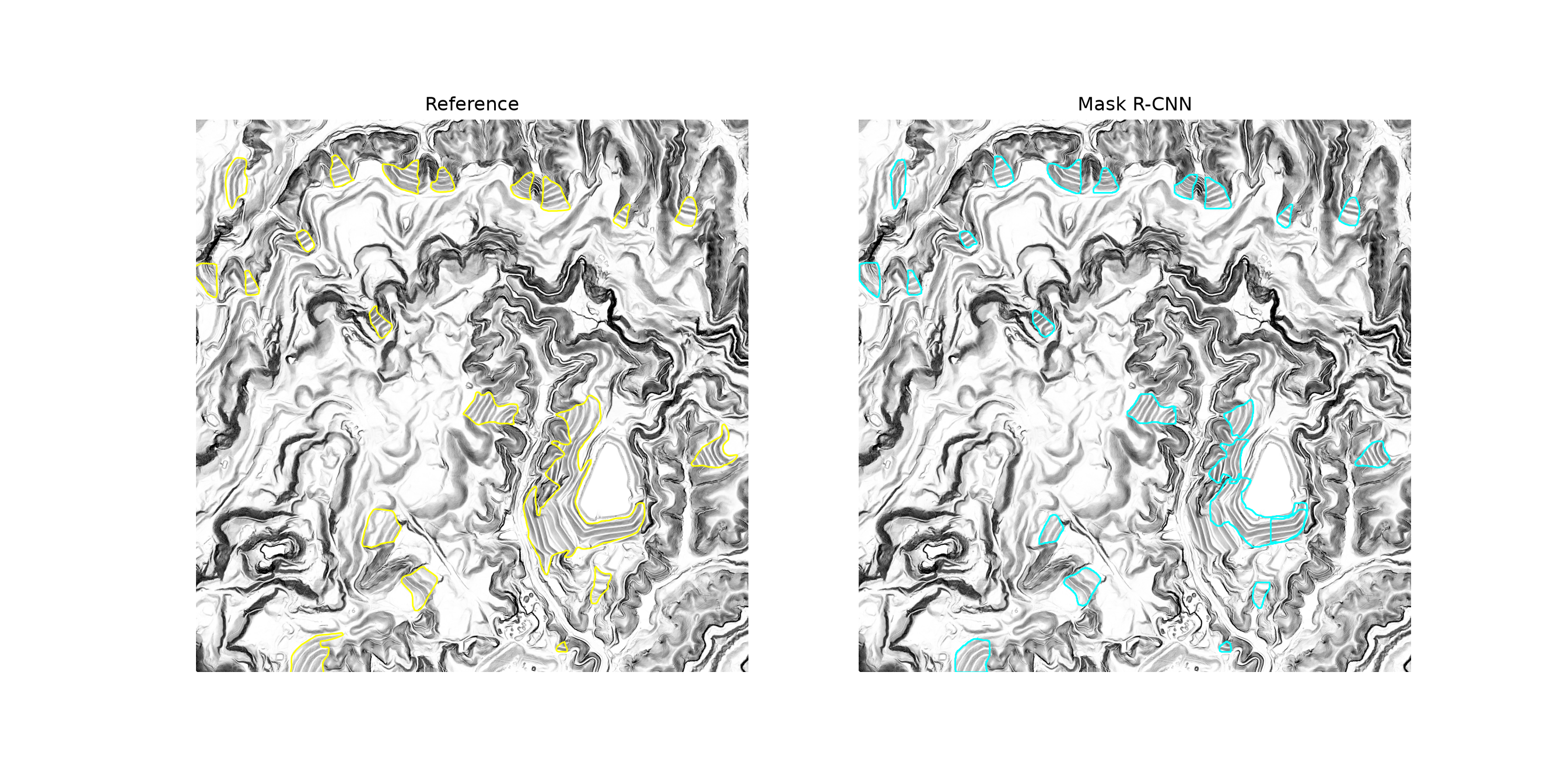
For this area, 23 valley fill faces were predicted, compared to 20 reference valley fill faces that intersect the area. Most of the reference valley fill faces were detected, and their predicted boundaries generally follow the reference boundaries, although the low-resolution masks produce somewhat smoothed outlines. Most of the errors occur in the large, complex mined area in the center, where several adjacent predictions only partially correspond to the reference polygons.
To assess the map, I rasterize each predicted and reference polygon to a binary mask aligned with the area and calculate the object-level metrics using the objectMetrics() function defined above. As for the chips, reference objects smaller than 200 cells are removed; these are slivers of valley fill faces that extend beyond the area. Since all predictions in predGDF already have a score of at least 0.5, the score threshold is set to 0. This is the same assessment used for the UNet-ID map in Chapter 22, so the results can be compared directly.
def polysToMasks(geoms, outShape, transform):
    return torch.stack([torch.from_numpy(features.rasterize([g], out_shape=outShape,
                                                            transform=transform)) for g in geoms])

predMasks = polysToMasks(predGDF.geometry, hillshade.shape, areaTransform)
refMasks = polysToMasks(refArea.geometry, hillshade.shape, areaTransform)
refMasks = refMasks[refMasks.flatten(1).sum(1) >= 200]
objectMetrics([{"masks": predMasks, "scores": torch.ones(len(predMasks))}],
              [{"masks": refMasks}], scoreThresh=0)
{'Precision': 0.739, 'Recall': 0.85, 'F1': 0.791}For the map area, 17 of the 23 predictions were matched to one of the 20 reference valley fill faces, for a precision of 0.739, a recall of 0.850, and an F1-score of 0.791. As for UNet-ID, these results are much better than those for the test chips, since few valley fill faces are cut by the edges of the area.
The result can be saved to a vector file using the GeoDataFrame’s to_file() method. For larger areas, the DTM can be processed in blocks, each with a buffer, and the polygons from all blocks combined, again removing duplicates along the block boundaries.
23.8 Comparing Mask R-CNN and UNet-ID
| UNet-ID (segmentation-based) | Mask R-CNN (detection-based) | |
|---|---|---|
| Instance separation | Post-processing (markers and watershed) | Direct: one prediction per object |
| Output resolution | Full-resolution masks | Masks predicted at low resolution (28x28) and resized |
| Object sizes | Handles irregular and very large objects well | Best for compact objects; very large or elongated objects are harder |
| Dense, touching objects | Depends on border prediction quality | Handles well, up to the maximum detections per image |
| Confidence scores | Per pixel | Per object, enabling AP-based assessment |
| Input bands | Any number of bands | Three bands, unless the backbone and normalization are adapted |
| Large-area mapping | Overlapping predictions cropped and mosaicked | Duplicate detections must be removed |
For the valley fill data, the two approaches performed similarly, as summarized below. For the VA1 test chips, Mask R-CNN, with a score threshold of 0.5, obtained a slightly higher object-level F1-score than UNet-ID, mostly due to its higher recall. For the 4x4 km map area, both approaches matched 17 of the 20 reference valley fill faces and produced 6 false positives. UNet-ID required a longer training time, about 73 minutes for 50 epochs compared to 39 minutes for 30 epochs for Mask R-CNN, but it was trained from scratch, while Mask R-CNN started from weights pre-trained on COCO. Given the small number of test objects, especially within the map area, these differences should not be overinterpreted.
| UNet-ID | Mask R-CNN | |
|---|---|---|
| Test chips: precision | 0.469 | 0.475 |
| Test chips: recall | 0.443 | 0.508 |
| Test chips: F1-score | 0.456 | 0.491 |
| Map area: precision | 0.739 | 0.739 |
| Map area: recall | 0.850 | 0.850 |
| Map area: F1-score | 0.791 | 0.791 |
Neither approach is universally better. Mask R-CNN’s low-resolution masks can produce smoothed or rounded boundaries, while UNet-ID’s full-resolution predictions capture boundaries in more detail but depend on a hand-designed post-processing step. The valley fill faces in this dataset do not touch each other, so they do not exercise one of Mask R-CNN’s main advantages, the separation of touching objects. They are also large and irregular, which favors full-resolution predictions. Comparing the two approaches on your own data, using object-level metrics, is a good way to choose.
23.9 Concluding Remarks
In this chapter, we explored Mask R-CNN, a detection-based instance segmentation architecture, using the torchvision implementation. We prepared data in the format expected by the torchvision detection models, adapted a pre-trained model to our classes and to LSP data, trained it using PyTorch Lightning, assessed it using mean average precision and object-level metrics, and mapped valley fill faces across a larger area while removing duplicate detections. In the next chapter, we return to semantic segmentation and explore ConvNeXt, a modern CNN architecture that incorporates design ideas from transformers.
23.10 Questions
- Explain the difference between object detection and instance segmentation. What does Mask R-CNN add to the Faster R-CNN architecture?
- Describe the roles of the feature pyramid network, the region proposal network, RoIAlign, the box head, and the mask head in Mask R-CNN.
- What are anchor boxes, and why are anchors with different sizes and aspect ratios used?
- Describe the format of the target dictionaries expected by the torchvision detection models. Why is class code 0 reserved, and how must an image containing no objects be represented?
- Why is a custom collate function required in the DataLoader when training Mask R-CNN?
- Explain how the behavior of the torchvision Mask R-CNN model differs between training and evaluation modes, and how this affects the LightningModule.
- Explain how average precision is calculated. What is the difference between AP50, AP75, and mAP calculated over IoU thresholds from 0.5 to 0.95?
- Why can duplicate detections occur when predicting a large area as overlapping chips, and how can they be removed?